10 DNA methylation analysis using bisulfite sequencing data
The epigenome consists of chemical modifications of DNA and histones. These modifications are shown to be associated with gene regulation in various settings (see Chapter 1 for an intro). These modifications in turn have specific importance for cell type identification. There are many different ways of measuring such modifications. We have shown how histone modifications can be measured in a genome-wide manner in Chapter 9 using ChIP-seq. In this chapter we will focus on the analysis of DNA methylation data using data from a technique called bisulfite sequencing (BS-seq). We will introduce how to process data and data quality checks, as well as statistical analysis relevant for BS-seq data.
10.1 What is DNA methylation?
Cytosine methylation (5-methylcytosine, 5mC) is one of the main covalent base modifications in eukaryotic genomes, generally observed on CpG dinucleotides. Methylation can also rarely occur in a non-CpG context, but this was mainly observed in human embryonic stem and neuronal cells (Lister et al. 2009; Lister et al. 2013). DNA methylation is a part of the epigenetic regulation mechanism of gene expression. It is cell-type-specific DNA modification. It is reversible but mostly remains stable through cell division. There are roughly 28 million CpGs in the human genome, 60–80% are generally methylated. Less than 10% of CpGs occur in CG-dense regions that are termed CpG islands in the human genome (Smith and Meissner 2013). It has been demonstrated that DNA methylation is also not uniformly distributed over the genome, but rather is associated with CpG density. In vertebrate genomes, cytosine bases are usually unmethylated in CpG-rich regions such as CpG islands and tend to be methylated in CpG-deficient regions. Vertebrate genomes are largely CpG deficient except at CpG islands. Conversely, invertebrates such as Drosophila melanogaster and Caenorhabditis elegans do not exhibit cytosine methylation and consequently do not have CpG rich and poor regions but rather a steady CpG frequency over their genomes (Deaton and Bird 2011).
10.1.1 How DNA methylation is set?
DNA methylation is established by DNA methyltransferases DNMT3A and DNMT3B in combination with DNMT3L and maintained through cell division by the methyltransferase DNMT1 and associated proteins. DNMT3a and DNMT3b are in charge of the de novo methylation during early development. Loss of 5mC can be achieved passively by dilution during replication or exclusion of DNMT1 from the nucleus. Recent discoveries of the ten-eleven translocation (TET) family of proteins and their ability to convert 5-methylcytosine (5mC) into 5-hydroxymethylcytosine (5hmC) in vertebrates provide a path for catalyzed active DNA demethylation (Tahiliani et al. 2009). Iterative oxidations of 5hmC catalyzed by TET result in 5-formylcytosine (5fC) and 5-carboxylcytosine (5caC). 5caC mark is excised from DNA by G/T mismatch-specific thymine-DNA glycosylase (TDG), which as a result reverts cytosine residue to its unmodified state (He et al. 2011). Apart from these, mainly bacteria, but possibly higher eukaryotes, contain base modifications on bases other than cytosine, such as methylated adenine or guanine (Clark et al. 2011).
10.1.2 How to measure DNA methylation with bisulfite sequencing
One of the most reliable and popular ways to measure DNA methylation is high-throughput bisulfite sequencing. This method, and the related ones, allow measurement of DNA methylation at the single nucleotide resolution. The bisulfite conversion turns unmethylated Cs to Ts and methylated Cs remain intact. Then, the only thing to do is to align the reads with those C->T conversions and count C->T mutations to calculate fraction of methylated bases. In the end, we can get quantitative genome-wide measurements for DNA methylation.
10.2 Analyzing DNA methylation data
For the remainder of this chapter, we will explain how to do DNA methylation analysis using R. The analysis process is somewhat similar to the analysis patterns observed in other sequencing data analyses. The process can be chunked to four main parts with further sub-chunks:
- Processing raw data
- Quality check
- Alignment and post-alignment processing
- Methylation calling
- Filtering bases
- Exploratory analysis
- Clustering
- PCA
- Finding interesting regions
- Differential methylation
- Methylation segmentation
- Annotating interesting regions
- Nearest genes
- Annotation with other genomic features
- Integration with other quantitative genomics data
10.3 Processing raw data and getting data into R
The rawest form of data that most users get is probably in the form of fastq files obtained from the sequencing experiments. We will describe the necessary steps and the tools that can be used for raw data processing and if they exist, we will mention their R equivalents. However, the data processing is usually done outside of the R framework, and for the following sections we will assume that the data processing is done and our analysis is starting from methylation call files.
The typical data processing step starts with a data quality check. The fastq files are first run through quality check software that shows the quality of the sequencing run. We would typically use fastQC for this. However, there are several bioconductor packages that could be of use, such as Rqc and QuasR. We have introduced how to use some of these tools for sequencing quality check in Chapter 7. Following the quality check, provided everything is OK, the reads can be aligned to the genome. Before the alignment, adapters or low-quality ends of the reads can be trimmed to increase number of alignments. Low-quality ends mostly likely have poor basecalls, which will lead to many mismatches. Reads with non-trimmed adapters will also not align to the genome. We would use adapter trimming tools such as cutadapt or flexbar for this purpose, although there are a bunch of them to choose from. Following this, reads are aligned to the genome with a bisulfite-treatment-aware aligner. For our own purposes, we use Bismark(Krueger and Andrews 2011), however there are other equally accurate aligners, and some are reviewed here. In addition, the Bioconductor package QuasR can align BS-seq reads within the R framework.
After alignment, we need to call C->T conversions and calculate the fraction/percentage of methylation. Most of the time, aligners come with auxiliary tools that calculate per-base methylation values. Normally, they output a tabular format containing the location of the Cs and methylation value and strand. Within R, QuasR} and methylKit }can call methylation values from BAM files albeit with some limitations. In essence, these methylation call files can be easily read into R and downstream analysis within R starts from that point. An important quality measure at this stage is to look at the conversion rate. This simply means how many unmethylated Cs are converted to Ts. Since we expect non-CpG methylation to be rare, we can simply count the number of C->T conversions in the non-CpG context and calculate conversion rate. The best way to do this would be via spike-in sequences where we expect no methylation at all. Since non-CpG methylation is tissue specific, calculating the conversion rate using non-CpG Cs might be misleading in some cases.
10.4 Data filtering and exploratory analysis
We assume that we start the analysis in R with the methylation call files. We will read those files in and carry out exploratory analysis, and we will show how to filter bases or regions from the data and in what circumstances we might need to do so. We will use the methylKit(Akalin et al. 2012) package for the bulk of the analysis. }
10.4.1 Reading methylation call files
A typical methylation call file looks like this:
##         chrBase   chr    base strand coverage freqC  freqT
## 1 chr21.9764539 chr21 9764539      R       12 25.00  75.00
## 2 chr21.9764513 chr21 9764513      R       12  0.00 100.00
## 3 chr21.9820622 chr21 9820622      F       13  0.00 100.00
## 4 chr21.9837545 chr21 9837545      F       11  0.00 100.00
## 5 chr21.9849022 chr21 9849022      F      124 72.58  27.42
Most of the time bisulfite sequencing experiments have test and control samples. The test samples can be from a disease tissue while the control samples can be from a healthy tissue. You can read a set of methylation call files that have test/control conditions giving a treatment vector option. The treatment vector defines the sample groups and it is very important for the differential methylation analysis. For the sake of subsequent analysis, file.list, sample.id and treatment option should have the same order. In the following example, the first two files have the sample IDs “test1” and “test2” and as determined by the treatment vector they belong to the same group. The third and fourth files have sample IDs “ctrl1” and “ctrl2” and they belong to the same group as indicated by the treatment vector. We will first get a list of file paths and have a look at the content.
library(methylKit)
file.list = list( system.file("extdata",
                             "test1.myCpG.txt", package = "methylKit"),
                 system.file("extdata",
                             "test2.myCpG.txt", package = "methylKit"),
                 system.file("extdata",
                             "control1.myCpG.txt", package = "methylKit"),
                 system.file("extdata",
                             "control2.myCpG.txt", package = "methylKit") )
If you look what is inside the file.list variable, you will see that it is a simple list of file paths. Each file contains methylation calls for a given sample. Now, we can read the files with the methRead() function.
# read the files to a methylRawList object: myobj
myobj=methRead(file.list,
           sample.id=list("test1","test2","ctrl1","ctrl2"),
           assembly="hg18",
           treatment=c(1,1,0,0),
           context="CpG"
           )
Tab-separated bedgraph like formats from Bismark methylation caller can also be read in by methylkit. In those cases, we have to provide either pipeline="bismarkCoverage" or pipeline="bismarkCytosineReport" to the methRead() function. In addition to the options we mentioned above, any tab-separated text file with a generic format can be read in using methylKit, such as methylation ratio files from BSMAP. See here for an example.
Before we move on, let us have a look at what kind of information is stored in myobj. This is technically a methylRawList object, which is essentially a list of methylRaw objects. These objects hold the information for the genomic location of Cs, and methylated Cs and unmethylated Cs.
## inside the methylRawList object
length(myobj)
## [1] 4head(myobj[[1]])## chr start end strand coverage numCs numTs
## 1 chr21 9764513 9764513 - 12 0 12
## 2 chr21 9764539 9764539 - 12 3 9
## 3 chr21 9820622 9820622 + 13 0 13
## 4 chr21 9837545 9837545 + 11 0 11
## 5 chr21 9849022 9849022 + 124 90 34
## 6 chr21 9853296 9853296 + 17 10 710.4.2 Further quality check
It is always a good idea to check how the data looks before proceeding further. For example, the methylation values should have bimodal distribution generally. This can be checked via the getMethylationStats() function. Normally, we should see bimodal distributions. Strong deviations from the bimodality may be due to poor experimental quality, such as problems with bisulfite treatment. Below we show how to get these plots using the getMethylationStats() function. The result is shown in Figure 10.1. As expected, it has a bimodal distribution where most CpGs have either high methylation or low methylation.
getMethylationStats(myobj[[2]],plot=TRUE,both.strands=FALSE)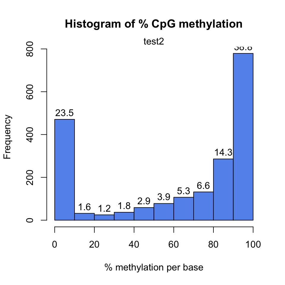
In addition, we might want to see coverage values. By default, methylkit handles bases with at least 10X coverage but that can be changed. The bases with unusually high coverage are usually alarming. It might indicate a PCR bias issue in the experimental procedure. The general coverage statistics can be checked with the getCoverageStats() function shown below. The resulting plot is shown in Figure 10.2.
getCoverageStats(myobj[[2]],plot=TRUE,both.strands=FALSE)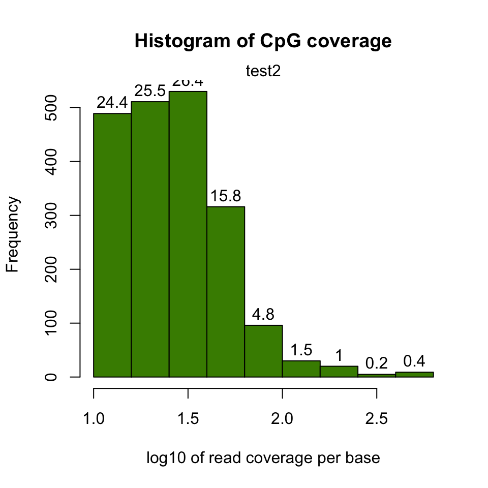
It might be useful to filter samples based on coverage. Particularly, if our samples are suffering from PCR bias, it would be useful to discard bases with very high read coverage. Furthermore, we would also like to discard bases that have low read coverage; a high enough read coverage will increase the power of the statistical tests. The code below filters a methylRawList, discards bases that have coverage below 10X, and also discards the bases that have more than 99.9th percentile of coverage in each sample.
filtered.myobj=filterByCoverage(myobj,lo.count=10,lo.perc=NULL,
                                      hi.count=NULL,hi.perc=99.9)
10.4.3 Merging samples into a single table
When we first read the files, each file is stored as its own entity. If we want to compare samples in any way, we need to make a unified data structure that contains CpGs that are covered in most samples. The unite() function creates a new object using the CpGs covered in each sample.
## we use :: notation to make sure unite() function from methylKit is called
meth=methylKit::unite(myobj, destrand=FALSE)
Let us take a look at the data content of the methylBase object:
head(meth)## chr start end strand coverage1 numCs1 numTs1 coverage2 numCs2 numTs2
## 1 chr21 9853296 9853296 + 17 10 7 333 268 65
## 2 chr21 9853326 9853326 + 17 12 5 329 249 79
## 3 chr21 9860126 9860126 + 39 38 1 83 78 5
## 4 chr21 9906604 9906604 + 68 42 26 111 97 14
## 5 chr21 9906616 9906616 + 68 52 16 111 104 7
## 6 chr21 9906619 9906619 + 68 59 9 111 109 2
## coverage3 numCs3 numTs3 coverage4 numCs4 numTs4
## 1 18 16 2 395 341 54
## 2 16 14 2 379 284 95
## 3 83 83 0 41 40 1
## 4 23 18 5 37 33 4
## 5 23 14 9 37 27 10
## 6 22 18 4 37 29 8By default, the unite() function produces bases/regions covered in all samples. That requirement can be relaxed using the min.per.group option in the unite() function.
# creates a methylBase object,
# where only CpGs covered with at least 1 sample per group will be returned

# there were two groups defined by the treatment vector,
# given during the creation of myobj: treatment=c(1,1,0,0)
meth.min=unite(myobj,min.per.group=1L)
10.4.4 Filtering CpGs
We might need to filter the CpGs further before exploratory analysis or even before the downstream analysis such as differential methylation. For exploratory analysis, it is of general interest to see how samples relate to each other and we might want to remove CpGs that are not variable before doing that. Or we might remove Cs that are potentially C->T mutations. First, we show how to filter based on variation. Below, we extract percent methylation values from CpGs as a matrix. Calculate the standard deviation for each CpG and filter based on standard deviation. We also plot the distribution of per-CpG standard deviations with the hist() function. The resulting plot is shown in Figure 10.3.
pm=percMethylation(meth) # get percent methylation matrix
mds=matrixStats::rowSds(pm) # calculate standard deviation of CpGs
head(meth[mds>20,])
## chr start end strand coverage1 numCs1 numTs1 coverage2 numCs2 numTs2
## 11 chr21 9906681 9906681 + 21 12 9 60 56 4
## 12 chr21 9906694 9906694 + 21 9 12 60 53 7
## 13 chr21 9906700 9906700 + 13 6 7 53 43 10
## 14 chr21 9906714 9906714 + 14 3 11 41 37 4
## 18 chr21 9906873 9906873 + 12 8 4 41 33 8
## 23 chr21 9927527 9927527 + 17 5 12 40 22 18
## coverage3 numCs3 numTs3 coverage4 numCs4 numTs4
## 11 37 14 23 26 11 15
## 12 39 16 23 26 15 11
## 13 30 8 22 23 10 13
## 14 25 19 6 21 19 2
## 18 15 4 11 22 7 15
## 23 32 32 0 14 11 3hist(mds,col="cornflowerblue",xlab="Std. dev. per CpG")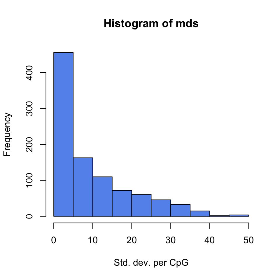
Now, let’s assume we know the locations of C->T mutations. These locations should be removed from the analysis as they do not represent bisulfite-treatment-associated conversions. Mutation locations are stored in a GRanges object, and we can use that to remove CpGs overlapping with mutations. In order to do the overlap operation, we will convert the methylKit object to a GRanges object and do the filtering with the %over% function within [ ]. The returned object will still be a methylKit object.
library(GenomicRanges)
# example SNP
mut=GRanges(seqnames=c("chr21","chr21"),
            ranges=IRanges(start=c(9853296, 9853326),
                           end=c( 9853296,9853326)))

# select CpGs that do not overlap with mutations
sub.meth=meth[! as(meth,"GRanges") %over% mut,]
nrow(meth)
## [1] 963nrow(sub.meth)## [1] 96110.4.5 Clustering samples
Clustering is used for grouping data points by their similarity. It is a general concept that can be achieved by many different algorithms and we introduced clustering and multiple prominent clustering algorithms in Chapter 4. In the context of DNA methylation, we are trying to find samples that are similar to each other. For example, if we sequenced 3 heart samples and 4 liver samples, we would expect liver samples will be more similar to each other than heart samples on the DNA methylation space.
The following function will cluster the samples and draw a dendrogram. It will use correlation distance, which is \(1-\rho\) , where \(\rho\) is the correlation coefficient between two pairs of samples. The cluster tree will be drawn using the “ward” method. This specific variant uses a “bottom up” approach: each data point starts in its own cluster, and pairs of clusters are merged as one moves up the hierarchy. In Ward’s method, two clusters are merged if the variance is minimized compared to other possible merge operations. This bottom up approach helps build the dendrogram showing the relationship between clusters. The result of the clustering is shown in Figure 10.4.
clusterSamples(meth, dist="correlation", method="ward", plot=TRUE)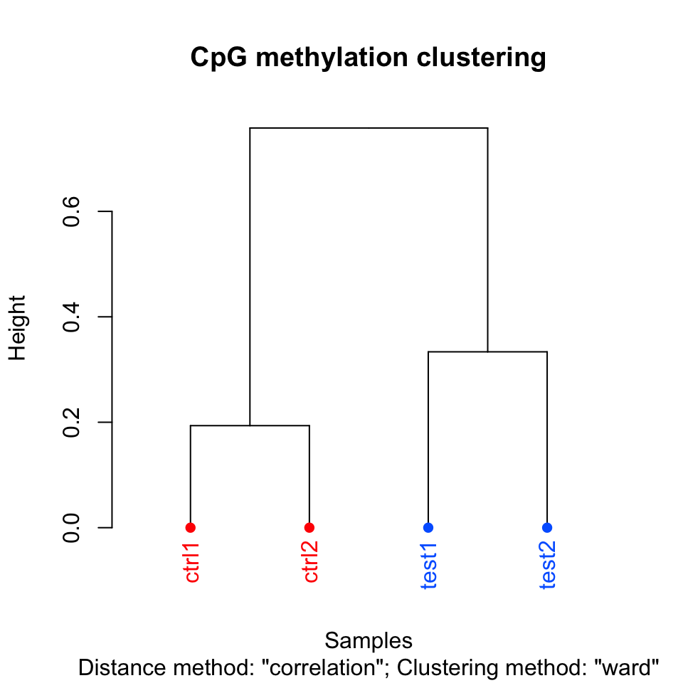
##
## Call:
## hclust(d = d, method = HCLUST.METHODS[hclust.method])
##
## Cluster method   : ward.D
## Distance         : pearson
## Number of objects: 4
Setting the plot=FALSE will return a dendrogram object which can be manipulated by users or fed in to other user functions that can work with dendrograms.
hc = clusterSamples(meth, dist="correlation", method="ward", plot=FALSE)10.4.6 Principal component analysis
Principal component analysis (PCA) is a mathematical transformation of (possibly) correlated variables into a number of uncorrelated variables called principal components. The resulting components from this transformation are defined in such a way that the first principal component has the highest variance and accounts for most of the variability in the data. We have introduced PCA and other similar methods in Chapter 4. The following function will plot a scree plot for importance of components and the result is shown in Figure 10.5.
PCASamples(meth, screeplot=TRUE)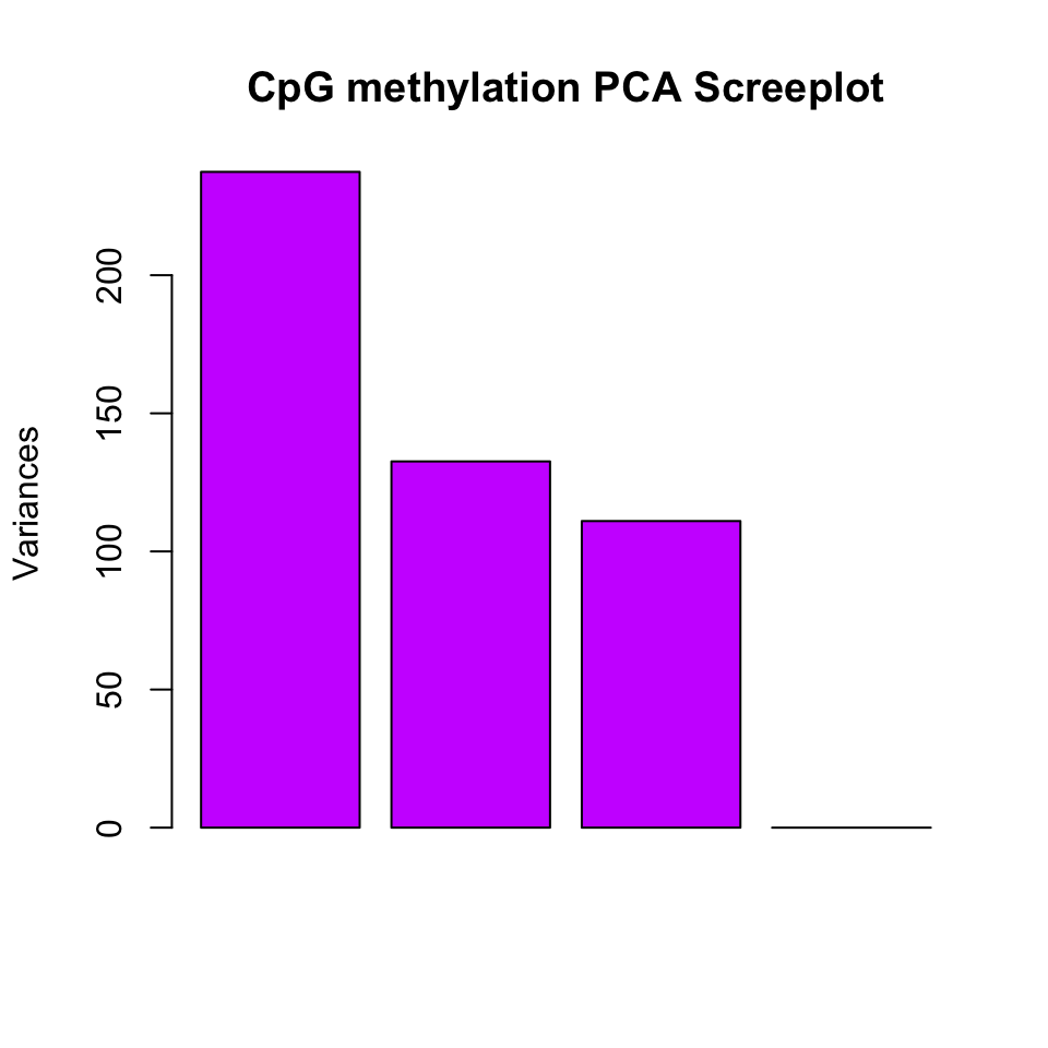
We can also plot the PC1 and PC2 axes and a scatter plot of our samples on those axes which will reveal how they cluster within these new dimensions. Similar to the clustering dendrogram, we would like to see samples that are similar to be close to each other on the scatter plot. If they are not, it might indicate problems with the experiment such as batch effects. The function below plots the samples in such a scatter plot on principal component axes. The resulting plot is shown in Figure 10.6.
pc=PCASamples(meth,obj.return = TRUE, adj.lim=c(1,1))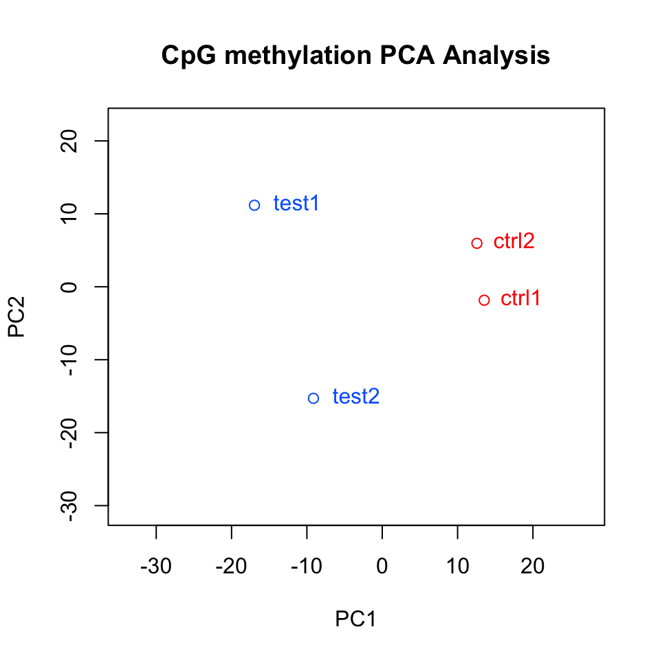
In this case, we also returned an object from the plotting function. This is the output of the prcomp() function, which includes loadings and eigenvectors which might be useful. You can also do your own PCA analysis using percMethylation() and prcomp(). In the case above, the methylation matrix is transposed. This allows us to compare distances between samples on the PCA scatter plot.
10.5 Extracting interesting regions: Differential methylation and segmentation
When analyzing DNA methylation data, we usually look for regions that are different than the rest of the methylome or different from a reference methylome. These regions are so-called “interesting regions”. They usually mark important genomic features that are related to gene regulation, which in turn defines the cell type. Therefore, it is a general interest to find such regions and analyze them further to understand our biological sample or to answer specific research questions. Below we will describe two ways of defining “regions of interest”.
10.5.1 Differential methylation
Once methylation proportions per base are obtained, generally, the differences between methylation profiles are considered next. When there are multiple sample groups where each group defines a separate biological entity or treatment, it is usually of interest to locate bases or regions with different methylation proportions across the sample groups. The bases or regions with different methylation proportions across samples are called differentially methylated CpG sites (DMCs) and differentially methylated regions (DMRs). They have been shown to play a role in many different diseases due to their association with epigenetic control of gene regulation. In addition, DNA methylation profiles can be highly tissue-specific due to their role in gene regulation (Schübeler 2015). DNA methylation is highly informative when studying normal and diseased cells, because it can also act as a biomarker. For example, the presence of large-scale abnormally methylated genomic regions is a hallmark feature of many types of cancers (Ehrlich 2002). Because of the aforementioned reasons, investigating differential methylation is usually one of the primary goals of doing bisulfite sequencing.
10.5.1.1 Fisher’s exact test
Differential DNA methylation is usually calculated by comparing the proportion of methylated Cs in a test sample relative to a control. In simple comparisons between such pairs of samples (i.e. test and control), methods such as Fisher’s exact test can be used. If there are replicates, replicates can be pooled within groups to a single sample per group. This strategy, however, does not take into account biological variability between replicates. We will now show how to compare pairs of samples via the calculateDiffMeth() function in methylKit. When there is only one sample per sample group, calculateDiffMeth() automatically applies Fisher’s exact test. We will now extract one sample from each group and run calculateDiffMeth(), which will automatically run Fisher’s exact test.
getSampleID(meth)
new.meth=reorganize(meth,sample.ids=c("test1","ctrl1"),treatment=c(1,0))
dmf=calculateDiffMeth(new.meth)
As mentioned, we can also pool the samples from the same group by adding up the number of Cs and Ts per group. This way even if we have replicated experiments we treat them as single experiments, and can apply Fisher’s exact test. We will now pool the samples and apply the calculateDiffMeth() function.
pooled.meth=pool(meth,sample.ids=c("test","control"))
dm.pooledf=calculateDiffMeth(pooled.meth)
The calculateDiffMeth() function returns the P-values for all bases or regions in the input methylBase object. We need to filter to get differentially methylated CpGs. This can be done via the getMethlyDiff() function or simple filtering via [ ] notation. Below we show how to filter the methylDiff object output by the calculateDiffMeth() function in order to get differentially methylated CpGs. The function arguments define cutoff values for the methylation difference between groups and q-value. In these cases, we require a methylation difference of 25% and a q-value of at least \(0.01\).
# get differentially methylated bases/regions with specific cutoffs
all.diff=getMethylDiff(dm.pooledf,difference=25,qvalue=0.01,type="all")

# get hyper-methylated
hyper=getMethylDiff(dm.pooledf,difference=25,qvalue=0.01,type="hyper")

# get hypo-methylated
hypo=getMethylDiff(dm.pooledf,difference=25,qvalue=0.01,type="hypo")

#using [ ] notation
hyper2=dm.pooledf[dm.pooledf$qvalue < 0.01 & dm.pooledf$meth.diff > 25,]
10.5.1.2 Logistic regression based tests
Regression-based methods are generally used to model methylation levels in relation to the sample groups and variation between replicates. Differences between currently available regression methods stem from the choice of distribution to model the data and the variation associated with it. In the simplest case, linear regression can be used to model methylation per given CpG or loci across sample groups. The model fits regression coefficients to model the expected methylation proportion values for each CpG site across sample groups. Hence, the null hypothesis of the model coefficients being zero could be tested using t-statistics. However, linear-regression-based methods might produce fitted methylation levels outside the range \([0,1]\) unless the values are transformed before regression. An alternative is logistic regression, which can deal with data strictly bounded between 0 and 1 and with non-constant variance, such as methylation proportion/fraction values. In the logistic regression, it is assumed that fitted values have variation \(np(1-p)\), where \(p\) is the fitted methylation proportion for a given sample and \(n\) is the read coverage. If the observed variance is larger or smaller than assumed by the model, one speaks of under- or over-dispersion. This over/under-dispersion can be corrected by calculating a scaling factor and using that factor to adjust the variance estimates as in \(np(1-p)s\), where \(s\) is the scaling factor. MethylKit can apply logistic regression to test the methylation difference with or without the over-dispersion correction. In this case, Chi-square or F-test can be used to compare the difference in the deviances of the null model and the alternative model. The null model assumes there is no relationship between sample groups and methylation, and the alternative model assumes that there is a relationship where sample groups are predictive of methylation values for a given CpG or region for which the model is constructed. Next, we are going to use the logistic-regression-based model with over-dispersion correction and Chi-square test.
dm.lr=calculateDiffMeth(meth,overdispersion = "MN",test ="Chisq")10.5.1.3 Betabinomial-distribution-based tests
More complex regression models use beta binomial distribution and are particularly useful for better modeling the variance. Similar to logistic regression, their observation follows binomial distribution (number of reads), but methylation proportion itself can vary across samples, according to a beta distribution. It can deal with fitting values in the \([0,1]\) range and performs better when there is greater variance than expected by the simple logistic model. In essence, these models have a different way of calculating a scaling factor when there is over-dispersion in the model. Further enhancements are made to these models by using the empirical Bayes methods that can better estimate hyper parameters of the beta distribution (variance-related parameters) by borrowing information between loci or regions within the genome to aid with inference about each individual loci or region. We are now going to use a beta-binomial based model called DSS (Feng et al. 2014) to calculate differential methylation.
dm.dss=calculateDiffMethDSS(meth)## Using internal DSS code...10.5.1.4 Differential methylation for regions rather than base-pairs
Until now, we have worked on differentially methylated cytosines. However, working with base-pair resolution data has its problems. Not all the CpGs will be covered in all samples. If covered they may have low coverage, which reduces the power of the tests. Instead of base-pairs, we can choose to work with regions. So, it might be desirable to summarize methylation information over pre-defined regions rather than doing base-pair resolution analysis. methylKit provides functionality to do such analysis. We can either tile the whole genome to tiles with predefined length, or we can use pre-defined regions such as promoters or CpG islands. This kind of regional analysis is carried out by adding up C and T counts from each covered cytosine and returning a total C and T count for each region.
The function below tiles the genome with windows of \(1000\) bp length and \(1000\) bp step-size and summarizes the methylation information on those tiles. In this case, it returns a methylRawList object which can be fed into unite() and calculateDiffMeth() functions consecutively to get differentially methylated regions.
tiles=tileMethylCounts(myobj,win.size=1000,step.size=1000)
head(tiles[[1]],3)
## chr start end strand coverage numCs numTs
## 1 chr21 9764001 9765000 * 24 3 21
## 2 chr21 9820001 9821000 * 13 0 13
## 3 chr21 9837001 9838000 * 11 0 11In addition, if we are interested in particular regions, we can also get those regions as methylKit objects after summarizing the methylation information as described above. The code below summarizes the methylation information over a given set of promoter regions and outputs a methylRaw or methylRawList object depending on the input. We are using the output of genomation functions used above to provide the locations of promoters. For regional summary functions, we need to provide regions of interest as GRanges objects}.
library(genomation)

# read the gene BED file
gene.obj=readTranscriptFeatures(system.file("extdata", "refseq.hg18.bed.txt",
                                           package = "methylKit"))
promoters=regionCounts(myobj,gene.obj$promoters)

head(promoters[[1]])
## chr start end strand coverage numCs numTs
## 1 chr21 10011791 10013791 - 7953 6662 1290
## 2 chr21 10119796 10121796 - 1725 1171 554
## 3 chr21 10119808 10121808 - 1725 1171 554
## 4 chr21 13903368 13905368 + 10 10 0
## 5 chr21 14273636 14275636 - 282 220 62
## 6 chr21 14509336 14511336 + 1058 55 1003In addition, it is possible to cluster DMCs based on their proximity and direction of differential methylation. This can be achieved by the methSeg() function in methylKit. We will see more about the methSeg() function in the following section. But it can take the output of getMethylDiff() function and therefore can work on DMCs to get differentially methylated regions.
10.5.1.5 Adding covariates
Covariates can be included in the analysis as well in methylKit. The calculateDiffMeth() function will then try to separate the influence of the covariates from the treatment effect via the logistic regression model. In this case, we will test if the full model (model with treatment and covariates) is better than the model with the covariates only. If there is no effect due to the treatment (sample groups), the full model will not explain the data better than the model with covariates only. In calculateDiffMeth(), this is achieved by supplying the covariates argument in the format of a data.frame. Below, we simulate methylation data and add a data.frame for the age. The data frame can include more columns, and those columns can also be factor variables. The row order of the data.frame should match the order of samples in the methylBase object. Below we are showing an example of this using a simulated data set where methylation values of CpGs will be affected by the age of the sample.
covariates=data.frame(age=c(30,80,34,30,80,40))
sim.methylBase=dataSim(replicates=6,sites=1000,
                        treatment=c(rep(1,3),rep(0,3)),
                        covariates=covariates,
                        sample.ids=c(paste0("test",1:3),paste0("ctrl",1:3)))

my.diffMeth3=calculateDiffMeth(sim.methylBase,
                               covariates=covariates,
                               overdispersion="MN",
                               test="Chisq",mc.cores=1)
10.5.2 Methylation segmentation
The analysis of methylation dynamics is not exclusively restricted to differentially methylated regions across samples. Apart from this there is also an interest in examining the methylation profiles within the same sample. Usually, depressions in methylation profiles pinpoint regulatory regions like gene promoters that co-localize with CG-dense CpG islands. On the other hand, many gene-body regions are extensively methylated and CpG-poor (Bock et al. 2012). These observations would describe a bimodal model of either hyper- or hypomethylated regions depending on the local density of CpGs (Lövkvist et al. 2016). However, given the detection of CpG-poor regions with locally reduced levels of methylation (on average 30%) in pluripotent embryonic stem cells and in neuronal progenitors in both mouse and human, a different model also seems reasonable (Stadler et al. 2011a). These low-methylated regions (LMRs) are located distal to promoters, have little overlap with CpG islands, and are associated with enhancer marks such as p300 binding sites and H3K27ac enrichment.
Now we are going to try to segment a portion for the H1 human embryonic stem cell line. MethylKit }uses change-point analysis to segment the methylome. In change-point analysis, the change-points of a genome-wide methylation signal are recorded and the genome is partitioned into regions between consecutive change points. CpGs in each segment are similar to each other more than the following segment. After segmentation, methylKit function methSeg() identifies segments that are further clustered into segment classes using a mixture modeling approach. This clustering is based on only the average methylation level of the segments and allows the detection of distinct methylome features comparable to unmethylated regions (UMRs), lowly methylated regions (LMRs), and fully methylated regions (FMRs) mentioned in Stadler et al. (Stadler et al. 2011b). The code snippet below reads the methylation data from the H1 cell line as a GRanges object, and runs the segmentation with potentially up to classes of segments. Mixture modeling determines the optimal number of segments using a statistic called Bayesian information criterion (BIC). The BIC is a statistic based on model likelihood and helps us select the model that fits the data better. We have set the number of segment classes to try using the G=1:4 argument. The minSeg arguments are related to the minimum number of CpGs in the segments. The function methSeg() outputs a diagnostic plot for segmentation. This plot is shown in Figure 10.7. It shows methylation values and lengths of segments in each segment class, as well as the BIC for different numbers of segments.
# read methylation data

methFile=system.file("extdata","H1.chr21.chr22.rds",
                     package="compGenomRData")
mbw=readRDS(methFile)

# segment the methylation data
res=methSeg(mbw,minSeg=10,G=1:4,
            join.neighbours = TRUE)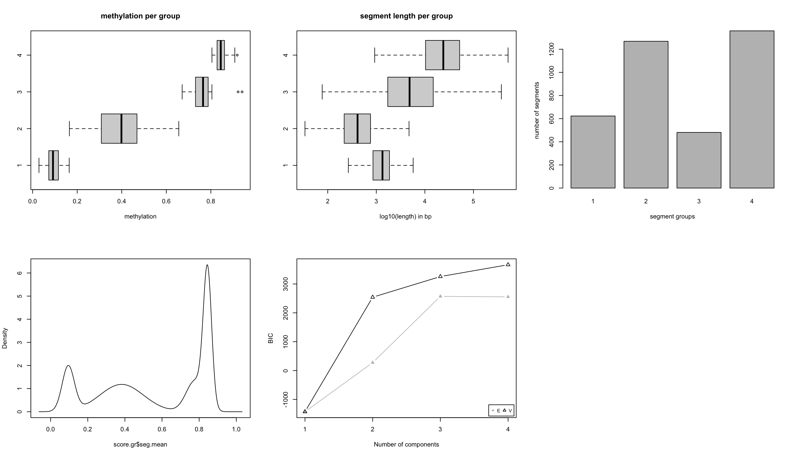
In this case, we know that BIC does not improve much after 4 segment classes. Now, we will not have a look at the characteristics of the segment classes. We are going to plot the mean methylation value and the length of the segment as a scatter plot; the result of this plot is shown in Figure 10.8.
# plot
plot(res$seg.mean,
     log10(width(res)),pch=20,
     col=scales::alpha(rainbow(4)[as.numeric(res$seg.group)], 0.2),
     ylab="log10(length)",
     xlab="methylation proportion")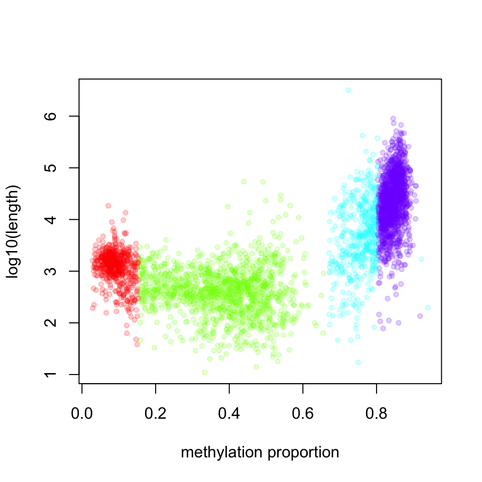
The highly methylated segment classes that have more than 70% methylation are usually longer; the median length is 17889 bp. The segment class that has the lowest methylation values have the median length of 1376 bp and the shortest segment class has low to medium methylation level, with median length of 412 bp.
10.5.3 Working with large files
We might want to perform differential methylation analysis in R using whole genome methylation data of multiple samples. The problem is that for genome-wide experiments, file sizes can easily range from hundreds of megabytes to gigabytes and processing multiple instances of those files in memory (RAM) might become unfeasible unless we have access to a high-performance compute cluster (HPC) with extensive RAM. If we want to use a desktop computer or laptop with limited RAM, we either need to restrict our analysis to a subset of the data or use packages that can handle this situation.
The methylKit package provides the capability of dealing with large files and high numbers of samples by exploiting flat file databases to substitute in-memory objects. The internal data, apart from meta information, has a tabular structure storing chromosome, start/end position, and strand information of the associated CpG base just like many other biological formats like BED, GFF or SAM. By exporting this tabular data into a TAB-delimited file and making sure it is accordingly position-sorted, it can be indexed using the generic tabix tool. In general, tabix indexing is a generalization of BAM indexing for generic TAB-delimited files. It inherits all the advantages of BAM indexing, including data compression and efficient random access in terms of few seek function calls per query (Li 2011). MethylKit relies on Rsamtools which implements tabix functionality for R. This way internal methylKit objects can be efficiently stored as a compressed file on the disk and still }be quickly accessed. Another advantage is that existing compressed files can be loaded in interactive sessions, allowing the backup and transfer of intermediate analysis results.
methylKit provides the capability for storing objects in tabix format within various functions. Every methylKit object has its tabix-based flat-file database equivalent. For example, when reading a methylation call file, the dbtype argument can be provided, which will create tabix-based objects.
 myobj=methRead( file.list,
               sample.id=list("test1","test2","ctrl1","ctrl2"),
               assembly="hg18",treatment=c(1,1,0,0),
               dbtype="tabix")
The advantage of tabix-based objects is of course saving memory and more efficient parallelization for differential methylation calculation. However, since the data is written to a file and indexed whenever a new object is created, working with tabix-based objects will be slower at certain steps of the analysis compared to in-memory objects.
10.6 Annotation of DMRs/DMCs and segments
The regions of interest obtained through differential methylation or segmentation analysis often need to be integrated with genome annotation datasets. Without this type of integration, differential methylation or segmentation results will be hard to interpret in biological terms. The most common annotation task is to see where regions of interest land in relation to genes and gene parts and regulatory regions: Do they mostly occupy promoter, intronic or exonic regions? Do they overlap with repeats? Do they overlap with other epigenomic markers or long-range regulatory regions? These questions are not specific to methylation −nearly all regions of interest obtained via genome-wide studies have to deal with such questions. Thus, there are already multiple software tools that can produce such annotations. One is the Bioconductor package genomation(Akalin et al. 2015). }It can be used to annotate DMRs/DMCs and it can also be used to integrate methylation proportions over the genome with other quantitative information and produce meta-gene plots or heatmaps. Below, we are reading a BED file for transcripts and using that to annotate DMCs with promoter/intron/exon/intergenic annotation. The genomation::readTranscriptFeatures() function reads a BED12 file, calculates the coordinates of promoters, exons, and introns and the subsequent function uses that information for annotation.
library(genomation)

# read the gene BED file
transcriptBED=system.file("extdata", "refseq.hg18.bed.txt",
                                           package = "methylKit")
gene.obj=readTranscriptFeatures(transcriptBED)
#
# annotate differentially methylated CpGs with
# promoter/exon/intron using annotation data
#
annotateWithGeneParts(as(all.diff,"GRanges"),gene.obj)
## promoter exon intron intergenic
## 28.24 15.27 33.59 58.02
## promoter exon intron intergenic
## 28.24 0.00 13.74 58.02
## promoter exon intron
## 0.29 0.03 0.17
## Min. 1st Qu. Median Mean 3rd Qu. Max.
## 5 815 49918 52410 94644 313528Similarly, we can read the CpG island annotation and annotate our differentially methylated bases/regions with them.
# read the shores and flanking regions and name the flanks as shores
# and CpG islands as CpGi
cpg.file=system.file("extdata", "cpgi.hg18.bed.txt",
                                        package = "methylKit")
cpg.obj=readFeatureFlank(cpg.file,
                           feature.flank.name=c("CpGi","shores"))
## Warning: 'GenomicRangesList' is deprecated.
## Use 'GRangesList(..., compress=FALSE)' instead.
## See help("Deprecated")#
# convert methylDiff object to GRanges and annotate
diffCpGann=annotateWithFeatureFlank(as(all.diff,"GRanges"),
cpg.obj$CpGi,cpg.obj$shores,
feature.name="CpGi",flank.name="shores")Besides these, DMRs/DMCs might be associated with changes in gene regulation. It might be desirable to overlap them with known transcription binding sites or motifs or histone modifications. These are simply overlap operations for these kinds of analysis. You can use the genomation::annotateWithFeature() function or any other approach shown in Chapter 6, and you can also do motif discovery with methods shown in Chapter 9.
10.6.1 Further annotation with genes or gene sets
The next obvious steps for annotating your DMRs/DMCs are figuring out which genes they are associated with. Figuring out which genes are associated with your regions of interest can give a better idea of the biological implications of the methylation changes. Once you have your gene set, you can do gene set analysis as shown in Chapter 8 or in Chapter 11. There are also packages such as rGREAT that can simultaneously associate DMRs or any other region of interest to genes and do gene set analysis.
10.7 Other R packages that can be used for methylation analysis
- DSS beta-binomial models with empirical Bayes for moderating dispersion.
- BSseq Regional differential methylation analysis using smoothing and linear-regression-based tests.
- BiSeq Regional differential methylation analysis using beta-binomial models.
- MethylSeekR: Methylome segmentation using HMM and cutoffs.
- QuasR: Methylation aware alignment and methylation calling, as well as fastQC-like fastq raw data quality check features.
10.8 Exercises
10.8.1 Differential methylation
The main objective of this exercise is getting differential methylated cytosines between two groups of samples: IDH-mut (AML patients with IDH mutations) vs. NBM (normal bone marrow samples).
- Download methylation call files from GEO. These files are readable by methlKit using default
methReadarguments. [Difficulty: Beginner]
| samples | Link |
|---|---|
| IDH1_rep1 | link |
| IDH1_rep2 | link |
| NBM_rep1 | link |
| NBM_rep2 | link |
Example code for reading a file:
library(methylKit)
m=methRead("~/Downloads/GSM919982_NBM_1_myCpG.txt.gz",
sample.id = "idh",assembly="hg18")- Find differentially methylated cytosines. Use chr1 and chr2 only if you need to save time. You can subset it after you download the files either in R or Unix. The files are for hg18 assembly of human genome. [Difficulty: Beginner]
- Describe the general differential methylation trend, what is the main effect for most CpGs? [Difficulty: Intermediate]
- Annotate differentially methylated cytosines (DMCs) as promoter/intron/exon? [Difficulty: Beginner]
- Which genes are the nearest to DMCs? [Difficulty: Intermediate]
- Can you do gene set analysis either in R or via web-based tools? [Difficulty: Advanced]
10.8.2 Methylome segmentation
The main objective of this exercise is to learn how to do methylome segmentation and the downstream analysis for annotation and data integration.
- Download the human embryonic stem-cell (H1 Cell Line) methylation bigWig files from the Roadmap Epigenomics website. It may take a while to understand how the website is structured and which bigWig file to use. That is part of the exercise. The files you will download are for hg19 assembly unless stated otherwise. [Difficulty: Beginner]
- Do segmentation on hESC methylome. You can only use chr1 if using the whole genome takes too much time. [Difficulty: Intermediate]
- Annotate segments and the kinds of gene-based features each segment class overlaps with (promoter/exon/intron). [Difficulty: Beginner]
- For each segment type, annotate the segments with chromHMM annotations from the Roadmap Epigenome database available here. The specific file you should use is here. This is a bed file with chromHMM annotations. chromHMM annotations are parts of the genome identified by a hidden-Markov-model-based machine learning algorithm. The segments correspond to active promoters, enhancers, active transcription, insulators, etc. The chromHMM model uses histone modification ChIP-seq and potentially other ChIP-seq data sets to annotate the genome.[Difficulty: Advanced]