11.4 Clustering using latent factors

A common analysis in biological investigations is clustering. This is often interesting in cancer studies as one hopes to find groups of tumors (clusters) which behave similarly, i.e. have similar risks and/or respond to the same drugs. PCA is a common step in clustering analyses, and so it is easy to see how the latent variable models above may all be a useful pre-processing step before clustering. In the examples below, we will use the latent variables inferred by the algorithms in the previous section on the set of colorectal cancer tumors from the TCGA. For a more complete introduction to clustering, see Chapter 4.

11.4.1 One-hot clustering

A specific clustering method for NMF data is to assume each sample is driven by one component, i.e. that the number of clusters \(K\) is the same as the number of latent variables in the model and that each sample may be associated to one of those components. We assign each sample a cluster label based on the latent variable which affects it the most. Figure 11.9 above (heatmap of 2-component NMF) shows the latent variable values for the two latent variables, for the 72 tumors, obtained by Joint NMF.

The two rows are the two latent variables, and the columns are the 72 tumors. We can observe that most tumors are indeed driven mainly by one of the factors, and not a combination of the two. We can use this to assign each tumor a cluster label based on its dominant factor, shown in the following code snippet, which also produces the heatmap in Figure 11.13.

# one-hot clustering in one line of code:
# assign each sample the cluster according to its dominant NMF factor
# easily accessible using the max.col function
nmf.clusters <- max.col(nmf.h)
names(nmf.clusters) <- rownames(nmf.h)

# create an annotation data frame indicating the NMF one-hot clusters
# as well as the cancer subtypes, for the heatmap plot below
anno_nmf_cl <- data.frame(
  nmf.cluster=factor(nmf.clusters),
  cms.subtype=factor(covariates[rownames(nmf.h),]$cms_label)
)

# generate the plot
pheatmap::pheatmap(t(nmf.h[order(nmf.clusters),]),
  cluster_cols=FALSE, cluster_rows=FALSE,
  annotation_col = anno_nmf_cl,
  show_colnames = FALSE,border_color=NA,
  main="Joint NMF factors\nwith clusters and molecular subtypes")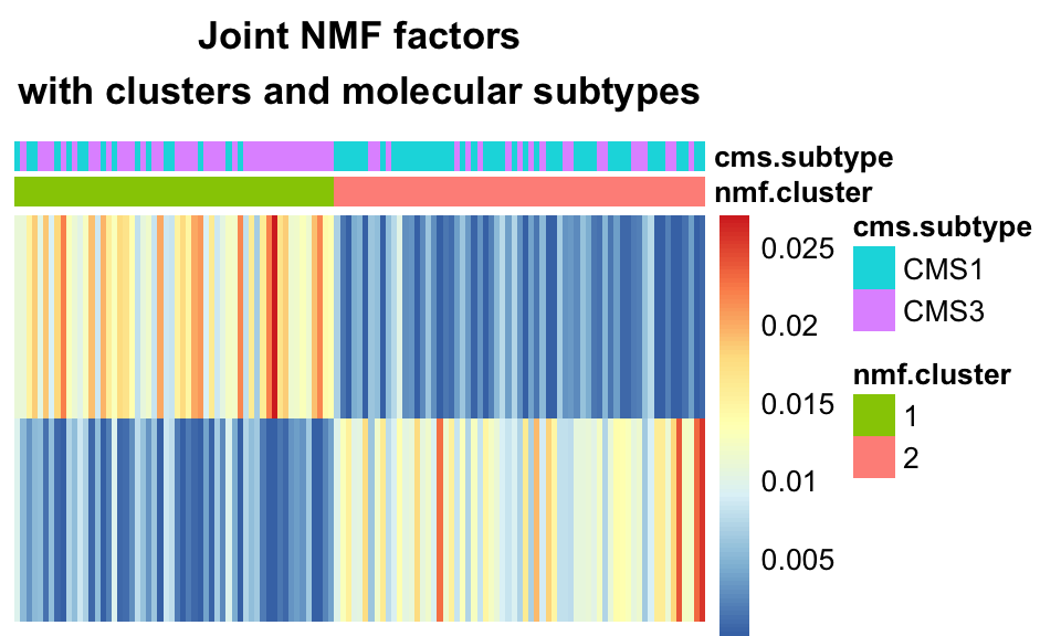

FIGURE 11.13: Joint NMF factors with clusters, and molecular sub-types. One-hot clustering assigns one cluster per dimension, where each sample is assigned a cluster based on its dominant component. The clusters largely recapitulate the CMS sub-types.

We see that using one-hot clustering with Joint NMF, we were able to find two clusters in the data which correspond fairly well with the molecular subtype of the tumors.

The one-hot clustering method does not lend itself very well to the other methods discussed above, i.e. iCluster and MFA. The latent variables produced by those other methods may be negative, and further, in the case of iCluster, are going to assume a multivariate Gaussian shape. As such, it is not trivial to pick one “dominant factor” for them. For NMF variants, this is a very common way to assign clusters.

11.4.2 K-means clustering

K-means clustering was introduced in Chapter 4. Briefly, k-means is a special case of the EM algorithm, and indeed iCluster was originally conceived as an extension of K-means from binary cluster assignments to real-valued latent variables. The iCluster algorithm, as it is so named, calls for application of K-means clustering on its latent variables, after the inference step. The following code snippet shows how to pull K-means clusters out of the iCluster results, and produces the heatmap in Figure 11.14, which shows how well these clusters correspond to cancer subtypes.

# use the kmeans function to cluster the iCluster H matrix (here, z)
# using 2 as the number of clusters.
icluster.clusters <- kmeans(icluster.z, 2)$cluster
names(icluster.clusters) <- rownames(icluster.z)

# create an annotation dataframe for the heatmap plot
# containing the kmeans cluster assignments and the cancer subtypes
anno_icluster_cl <- data.frame(
  iCluster=factor(icluster.clusters),
  cms.subtype=factor(covariates$cms_label))

# generate the figure
pheatmap::pheatmap(
  t(icluster.z[order(icluster.clusters),]), # order z by the kmeans clusters
  cluster_cols=FALSE, # use cluster_cols and cluster_rows=FALSE
  cluster_rows=FALSE, # as we want the ordering by k-means clusters to hold
  show_colnames = FALSE,border_color=NA,
  annotation_col = anno_icluster_cl,
  main="iCluster factors\nwith clusters and molecular subtypes")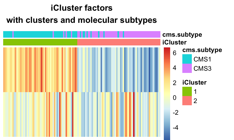

FIGURE 11.14: K-means clustering on iCluster+ factors largely recapitulates the CMS sub-types.

This demonstrates the ability of iClusterPlus to find clusters which correspond to molecular subtypes, based on multi-omics data.