5.13 Logistic regression and regularization
Logistic regression is a statistical method that is used to model a binary response variable based on predictor variables. Although initially devised for two-class or binary response problems, this method can be generalized to multiclass problems. However, our example tumor sample data is a binary response or two-class problem, therefore we will not go into the multiclass case in this chapter.
Logistic regression is very similar to linear regression as a concept and it can be thought of as a “maximum likelihood estimation” problem where we are trying to find statistical parameters that maximize the likelihood of the observed data being sampled from the statistical distribution of interest. This is also very related to the general cost/loss function approach we see in supervised machine learning algorithms. In the case of binary response variables, the simple linear regression model, such as \(y_i \sim \beta _{0}+\beta _{1}x_i\), would be a poor choice because it can easily generate values outside of the \(0\) to \(1\) boundary. What we need is a model that restricts the lower bound of the prediction to zero and an upper bound to \(1\). The first thing towards this requirement is to formulate the problem differently. If \(y_i\) can only be \(0\) or \(1\), we can formulate \(y_i\) as a realization of a random variable that can take the values one and zero with probabilities \(p_i\) and \(1-{p_i}\), respectively. This random variable follows the Bernoulli distribution, and instead of predicting the binary variable we can formulate the problem as \(p_i \sim \beta _{0}+\beta _{1}x_i\). However, our initial problem still stands, simple linear regression will still result in values that are beyond \(0\) and \(1\) boundaries. A model that satisfies the boundary requirement is the logistic equation shown below.
\[ {\displaystyle p_i={\frac {e^{(\beta _{0}+\beta _{1}x_i)}}{1+e^{(\beta _{0}+\beta_{1}x_i)}}}} \]
This equation can be linearized by the following transformation
\[ {\displaystyle \operatorname{logit} (p_i)=\ln \left({\frac {p_i}{1-p_i}}\right)=\beta _{0}+\beta _{1}x_i} \] The left-hand side is termed the logit, which stands for “logistic unit”. It is also known as the log odds. In this case, our model will produce values on the log scale and with the logistic equation above, we can transform the values to the \(0-1\) range. Now, the question remains: “What are the best parameter estimates for our training set”. Within the maximum likelihood framework we have touched upon in Chapter 3, the best parameter estimates are the ones that maximize the likelihood of the statistical model actually producing the observed data. You can think of this fitting as a probability distribution to an observed data set. The parameters of the probability distribution should maximize the likelihood that the observed data came from the distribution in question. If we were using a Gaussian distribution we would change the mean and variance parameters until the observed data was more plausible to be drawn from that specific Gaussian distribution.
In logistic regression, the response variable is modeled with a binomial distribution or its special case Bernoulli distribution. The value of each response variable, \(y_i\), is 0 or 1, and we need to figure out parameter \(p_i\) values that could generate such a distribution of 0s and 1s. If we can find the best \(p_i\) values for each tumor sample \(i\), we would be maximizing the log-likelihood function of the model over the observed data. The maximum log-likelihood function for our binary response variable case is shown as Equation (5.1).
\[\begin{equation} \operatorname{\ln} (L)=\sum_{i=1}^N\bigg[{\ln(1-p_i)+y_i\ln \left({\frac {p_i}{1-p_i}}\right)\bigg]} \tag{5.1} \end{equation}\]
In order to maximize this equation we have to find optimum \(p_i\) values which are dependent on parameters \(\beta_0\) and \(\beta_1\), and also dependent on the values of predictor variables \(x_i\). We can rearrange the equation replacing \(p_i\) with the logistic equation. In addition, many optimization functions minimize rather than maximize. Therefore, we will be using negative log likelihood, which is also called the “log loss” or “logistic loss” function. The function below is the “log loss” function. We substituted \(p_i\) with the logistic equation and simplified the expression.
\[\begin{equation} \operatorname L_{log}=-{\ln}(L)=-\sum_{i=1}^N\bigg[-{\ln(1+e^{(\beta _{0}+\beta _{1}x_i)})+y_i \left(\beta _{0}+\beta _{1}x_i\right)\bigg]} \tag{5.2} \end{equation}\]
Now, let us see how this works in practice. First, as in the example above we will use one predictor variable, the expression of one gene to classify tumor samples to “CIMP” and “noCIMP” subtypes. We will be using PDPN gene expression, which was one of the most important variables in our random forest model. We will use the formula interface in caret, where we will supply the names of the response and predictor variables in a formula. In this case, we will be using a core R function, glm(), from the stats package. “glm” stands for generalized linear models, and it is the main interface for different types of regression
in R.
# fit logistic regression model
# method and family defines the type of regression
# in this case these arguments mean that we are doing logistic
# regression
lrFit = train(subtype ~ PDPN,
               data=training, trControl=trainControl("none"),
               method="glm", family="binomial")

# create data to plot the sigmoid curve
newdat <- data.frame(PDPN=seq(min(training$PDPN),
                               max(training$PDPN),len=100))

# predict probabilities for the simulated data
newdat$subtype = predict(lrFit, newdata=newdat, type="prob")[,1]

# plot the sigmoid curve and the training data
plot(ifelse(subtype=="CIMP",1,0) ~ PDPN,
     data=training, col="red4",
     ylab="subtype as 0 or 1", xlab="PDPN expression")
lines(subtype ~ PDPN, newdat, col="green4", lwd=2)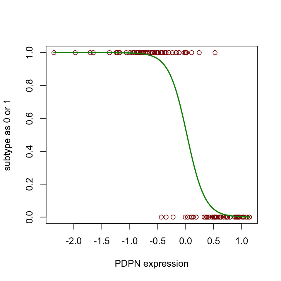
FIGURE 5.11: Sigmoid curve for prediction of subtype based on one predictor variable.
Figure 5.11 shows the sigmoidal curve that is fitted by the logistic regression. “noCIMP” subtype has higher expression of the PDPN gene than the “CIMP” subtype. In other words, the higher the values of PDPN, the more likely that the tumor sample will be classified as “noCIMP”. We can also assess the performance of our model with the test set and the training set. Let us try to do that again with the caret::predict() and caret::confusionMatrix() functions.
# training accuracy
class.res=predict(lrFit,training[,-1])
confusionMatrix(training[,1],class.res)$overall[1]
## Accuracy
## 0.9461538# test accuracy
class.res=predict(lrFit,testing[,-1])
confusionMatrix(testing[,1],class.res)$overall[1]## Accuracy
## 0.9259259The test accuracy is slightly worse than the training accuracy. Overall this is not as good as k-NN, but remember we used only one predictor variable. We have thousands of genes as predictor variables. Now we will try to use all of them in the classification problem. After fitting the model, we will check training and test accuracy. We fit the model again with the caret::train() function.
lrFit2 = train(subtype ~ .,
                data=training,
                # no model tuning with sampling
                trControl=trainControl("none"),
                method="glm", family="binomial")

# training accuracy
class.res=predict(lrFit2,training[,-1])
confusionMatrix(training[,1],class.res)$overall[1]
## Accuracy
## 1# test accuracy
class.res=predict(lrFit2,testing[,-1])
confusionMatrix(testing[,1],class.res)$overall[1]## Accuracy
## 0.4259259Training accuracy is \(1\), so training error is \(0\), and nothing is misclassified in the training set. However, test accuracy/error is close to terrible. It does only little better than a random guess. If we randomly assigned class labels we would get 0.5 accuracy. The test set accuracy is 0.55 despite the 100% training accuracy. This is because the model overfits to the training data. There are too many variables in the model. The number of predictor variables is ~6.5 times more than the number of samples. The excess of predictor variables makes the model very flexible (high variance), and this leads to overfitting.
5.13.1 Regularization in order to avoid overfitting
If we can limit the flexibility of the model, this might help with performance on the unseen, new data sets. Generally, any modification of the learning method to improve performance on the unseen datasets is called regularization. We need regularization to introduce bias to the model and to decrease the variance. This can be achieved by modifying the loss function with a penalty term which effectively shrinks the estimates of the coefficients. Therefore these types of methods within the framework of regression are also called “shrinkage” methods or “penalized regression” methods.
One way to ensure shrinkage is to add the penalty term, \(\lambda\sum{\beta_j}^2\), to the loss function. This penalty term is also known as the L2 norm or L2 penalty. It is calculated as the square root of the sum of the squared vector values. This term will help shrink the coefficients in the regression towards zero. The new loss function is as follows, where \(j\) is the number of parameters/coefficients in the model and \(L_{log}\) is the log loss function in Eq. (5.2).
\[\begin{equation} L_{log}+\lambda\sum_{j=1}^p{\beta_j}^2 \tag{5.3} \end{equation}\]
This penalized loss function is called “ridge regression” (Hoerl and Kennard 1970). When we add the penalty, the only way the optimization procedure keeps the overall loss function minimum is to assign smaller values to the coefficients. The \(\lambda\) parameter controls how much emphasis is given to the penalty term. The higher the \(\lambda\) value, the more coefficients in the regression will be pushed towards zero. However, they will never be exactly zero. This is not desirable if we want the model to select important variables. A small modification to the penalty is to use the absolute values of \(B_j\) instead of squared values. This penalty is called the “L1 norm” or “L1 penalty”. The regression method that uses the L1 penalty is known as “Lasso regression” (Tibshirani 1996).
\[ L_{log}+\lambda\sum_{j=1}^p{|\beta_j}| \] However, the L1 penalty tends to pick one variable at random when predictor variables are correlated. In this case, it looks like one of the variables is not important although it might still have predictive power. The Ridge regression on the other hand shrinks coefficients of correlated variables towards each other, keeping all of them. It has been shown that both Lasso and Ridge regression have their drawbacks and advantages (Friedman, Hastie, and Tibshirani 2010). More recently, a method called “elastic net” was proposed to include the best of both worlds (Zou and Hastie 2005). This method uses both L1 and L2 penalties. The equation below shows the modified loss function by this penalty. As you can see the \(\lambda\) parameter still controls the weight that is given to the penalty. This time the additional parameter \(\alpha\) controls the weight given to L1 or L2 penalty and it is a value between 0 and 1. \[ L_{log}+\lambda\sum_{j=1}^p{(\alpha\beta_j^2+(1-\alpha)|\beta_j}|) \]
We have now got the concept behind regularization and we can see how it works in practice. We are going to use elastic net on our tumor subtype prediction problem. We will let cross-validation select the best \(\lambda\) and we will fix the \(\alpha\) parameter at \(0.5\).
set.seed(17)
library(glmnet)

# this method controls everything about training
# we will just set up 10-fold cross validation
trctrl <- trainControl(method = "cv",number=10)

# we will now train elastic net model
# it will try
enetFit <- train(subtype~., data = training,
                 method = "glmnet",
                 trControl=trctrl,
                 # alpha and lambda paramters to try
                 tuneGrid = data.frame(alpha=0.5,
                                       lambda=seq(0.1,0.7,0.05)))

# best alpha and lambda values by cross-validation accuracy
enetFit$bestTune
## alpha lambda
## 1 0.5 0.1# test accuracy
class.res=predict(enetFit,testing[,-1])
confusionMatrix(testing[,1],class.res)$overall[1]## Accuracy
## 0.9814815As you can see regularization worked, the tuning step selected \(\lambda=1\), and we were able to get a satisfactory test set accuracy with the best model.
5.13.2 Variable importance
The variable importance of the penalized regression, especially for lasso and elastic net, is more or less out of the box. As discussed, these methods will set regression coefficients for irrelevant variables to zero. This provides a system for selecting important variables but it does not necessarily provide a way to rank them. Using the size of the regression coefficients is a way to rank predictor variables, however if the data is not normalized, you will get different scales for different variables. In our case, we normalized the data and we know that the variables have the same scale before they went into the training. We can use this fact and rank them based on the regression coefficients. The caret::varImp() function uses the coefficients to rank the variables from the elastic net model. Below, were going to plot the top 10 important variables which are normalized to the importance of the most important variable.
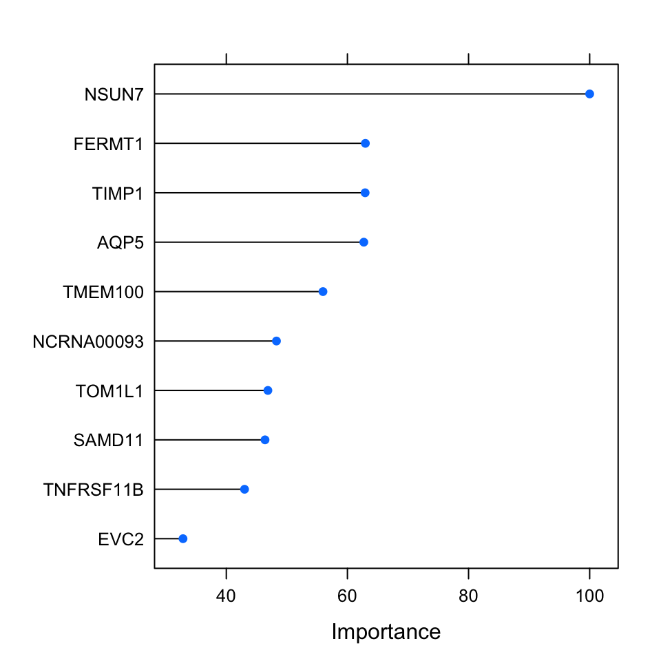
FIGURE 5.12: Variable importance metric for elastic net. This metric uses regression coefficients as importance.
Want to know more ?
- Lecture by Trevor Hastie on regularized regression. You probably need to understand the basics of regression and its terminology to follow this. However, the lecture is not very heavy on math. https://youtu.be/BU2gjoLPfDc
References
Friedman, Hastie, and Tibshirani. 2010. “Regularization Paths for Generalized Linear Models via Coordinate Descent.” Journal of Statistical Software 33 (1): 1.
Hoerl, and Kennard. 1970. “Ridge Regression: Biased Estimation for Nonorthogonal Problems.” Technometrics 12 (1): 55–67.
Tibshirani. 1996. “Regression Shrinkage and Selection via the Lasso.” Journal of the Royal Statistical Society: Series B (Methodological) 58 (1): 267–88.
Zou, and Hastie. 2005. “Regularization and Variable Selection via the Elastic Net.” Journal of the Royal Statistical Society: Series B (Statistical Methodology) 67 (2): 301–20.