5.8 Model tuning and avoiding overfitting

How can we know that we picked the best \(k\)? One straightforward way is that we can try many different \(k\) values and check the accuracy of our model. We will first check the effect of different \(k\) values on training accuracy. Below, we will go through many \(k\) values and calculate the training accuracy for each.

set.seed(101)
k=1:12 # set k values
trainErr=c() # set vector for training errors
for( i in k){
  
  knnFit=knn3(x=training[,-1], # training set
              y=training[,1], # training set class labels
              k=i)

  # predictions on the training set
  class.res=predict(knnFit,training[,-1],type="class")

  # training error
  err=1-confusionMatrix(training[,1],class.res)$overall[1]
  trainErr[i]=err
}

# plot training error vs k
plot(k,trainErr,type="p",col="#CC0000",pch=20)

# add a smooth line for the trend
lines(loess.smooth(x=k, trainErr,degree=2),col="#CC0000")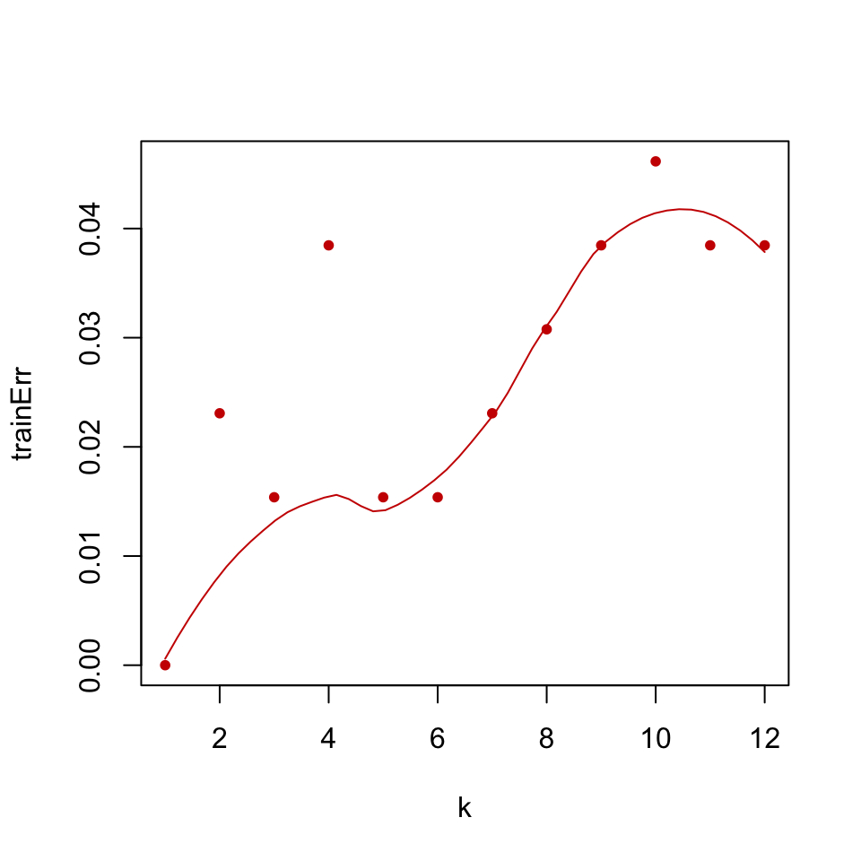

FIGURE 5.4: Training error for k-NN classification of glioma tumor samples.

The resulting training error plot is shown in Figure 5.4. We can see the effect of \(k\) in the training error; as \(k\) increases the model tends to be a bit worse on training. This makes sense because with large \(k\) we take into account more and more neighbors, and at some point we start considering data points from the other classes as well and that decreases our accuracy.

However, looking at the training accuracy is not the right way to test the model as we have mentioned. The models are generally tested on the datasets that are not used when building model. There are different strategies to do this. We have already split part of our dataset as test set, so let us see how we do it on the test data using the code below. The resulting plot is shown in Figure 5.5.

set.seed(31)
k=1:12
testErr=c()
for( i in k){

  knnFit=knn3(x=training[,-1], # training set
              y=training[,1], # training set class labels
              k=i)

  # predictions on the training set
  class.res=predict(knnFit,testing[,-1],type="class")
  testErr[i]=1-confusionMatrix(testing[,1],
                                 class.res)$overall[1]
 
}

# plot training error
plot(k,trainErr,type="p",col="#CC0000",
     ylim=c(0.000,0.08),
     ylab="prediction error (1-accuracy)",pch=19)
# add a smooth line for the trend
lines(loess.smooth(x=k, trainErr,degree=2), col="#CC0000")

# plot test error
points(k,testErr,col="#00CC66",pch=19) 
lines(loess.smooth(x=k,testErr,degree=2), col="#00CC66")
# add legend
legend("bottomright",fill=c("#CC0000","#00CC66"),
       legend=c("training","test"),bty="n")

FIGURE 5.5: Training and test error for k-NN classification of glioma tumor samples.

The test data show a different thing, of course. It is not the best strategy to increase the \(k\) indefinitely. The test error rate increases after a while. Increasing \(k\) results in too many data points influencing the decision about the class of the new sample, this may not be desirable since this strategy might include points from other classes eventually. On the other hand, if we set \(k\) too low, we are restricting the model to only look for a few neighbors.

In addition, \(k\) values that give the best performance for the training set are not the best \(k\) for the test set. In fact, if we stick with \(k=1\) as the best \(k\) obtained from the training set, we would obtain a worse performance on the test set. In this case, we can talk about the concept of overfitting. This happens when our models fit the data in the training set extremely well but cannot perform well in the test data; in other words, they cannot generalize. Similarly, underfitting could occur when our models do not learn well from the training data and they are overly simplistic. Ideally, we should use methods that help us estimate the real test error when tuning the models such as cross-validation, bootstrap or holdout test set.

5.8.1 Model complexity and bias variance trade-off

The case of over- and underfitting is closely related to the model complexity and the related bias-variance trade-off. We will introduce these concepts now. First, let us point out that prediction error depends on the real value of the class label of the test case and predicted value. The test case label or value is not dependent on the prediction; the only thing that is variable here is the model. Therefore, if we could train multiple models with different data sets for the same problem, our predictions for the test set would vary. That means our prediction error would also vary. Now, with this setting we can talk about expected prediction error for a given machine learning model. This is the average error you would get for a test set if you were able to train multiple models. This expected prediction error can largely be decomposed into the variability of the predictions due to the model variability (variance) and the difference between the expected prediction values and the correct value of the response (bias). Formally, the expected prediction error, \(E[Error]\) is decomposed as follows:

\[ E[Error]=Bias^2 + Variance + \sigma_e^2 \] Note that in the above equation \(\sigma_e^2\) is the irreducible error. This is the noise term that cannot fundamentally be accounted for by any model. The bias is formally the difference between the expected prediction value and the correct response value, \(Y\): \(Bias=(Y-E[PredictedValue])\). The variance is simply the variability of the prediction values when we construct models multiple times with different training sets for the same problem: \(Variance=E[(PredictedValue-E[PredictedValue])^2]\). Note that this value of the variance does not depend of the correct value of the test cases.

The models that have high variance are generally more complex models that have many knobs or parameters than can fit the training data well. These models, due to their flexibility, can fit training data too much that it creates poor prediction performance in a new data set. On the other hand, simple, less complex models do not have the flexibility to fit every data set that well, so they can avoid overfitting. However, they can underfit if they are not flexible enough to model or at least approximate the true relationship between predictors and the response variable. The bias term is mostly about the general model performance (expected or average value of predictions) that can be attributed to approximating a real-life problem with simpler models. These simple models can have less variability in their predictions, so the prediction error will be mostly composed of the bias term.

In reality, there is always a trade-off between bias and variance (See Figure 5.6). Increasing the variance with complex models will decrease the bias, but that might overfit. Conversely, simple models will increase the bias at the expense of the model variance, and that might underfit. There is an optimal point for model complexity, a balance between overfitting and underfitting. In practice, there is no analytical way to find this optimal complexity. Instead we must use an accurate measure of prediction error and explore different levels of model complexity and choose the complexity level that minimizes the overall error. Another approach to this is to use “the one standard error rule”. Instead of choosing the parameter that minimizes the error estimate, we can choose the simplest model whose error estimate is within one standard error of the best model (see Chapter 7 of (J. Friedman, Hastie, and Tibshirani 2001)). The rationale behind that is to choose a simple model with the hope that it would perform better in the unseen data since its performance is not different from the best model in a statistically significant way. You might see the option to choose the “one-standard-error” model in some machine learning packages.

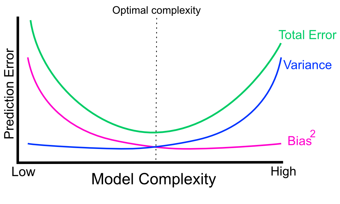
FIGURE 5.6: Variance-bias trade-off visualized as components of total prediction error in relation to model complexity.

In our k-NN example, lower \(k\) values create a more flexible model. This might be counterintuitive, but as we have explained before having small \(k\) values will fit the data in a very data-specific manner. It will probably not generalize well. Therefore in this respect, lower \(k\) values will result in more complex models with high variance. On the other hand, higher \(k\) values will result in less variance but higher bias. Figure 5.7 shows the decision boundary for two different k-NN models with \(k=2\) and \(k=12\). To be able to plot this in 2D we ran the model on principal component 1 and 2 of the training data set, and predicted the class label of many points in this 2D space. As you can see, \(k=2\) creates a more variable model which tries aggressively to include all training samples in the correct class. This creates a high-variance model because the model could change drastically from dataset to dataset. On the other hand, setting \(k=12\) creates a model with a smoother decision boundary. This model will have less variance since it considers many points for a decision, and therefore the decision boundary is smoother.

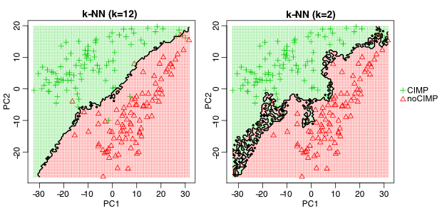
FIGURE 5.7: Decision boundary for different k values in k-NN models. k=12 creates a smooth decision boundary and ignores certain data points on either side of the boundary. k=2 is less smooth and more variable.

5.8.2 Data split strategies for model tuning and testing

The data split strategy is essential for accurate prediction of the test error. As we have seen in the model complexity/bias-variance discussion, estimating the prediction error is central for model tuning in order to find the model with the right complexity. Therefore, we will revisit this and show how to build and test models, and measure their prediction error in practice.

5.8.2.1 Training-validation-test

This data split strategy creates three partitions of the dataset, training, validation, and test sets. In this strategy, the training set is used to train the data and the validation set is used to tune the model to the best possible model. The final partition, “test”, is only used for the final test and should not be used to tune the model. This is regarded as the real-world prediction error for your model. This strategy works when you have a lot of data to do a three-way split. The test set we used above is most likely too small to measure the prediction error with just using a test set. In such cases, bootstrap or cross-validation should yield more stable results.

5.8.2.2 Cross-validation

A more realistic approach when you do not have a lot of data to do the three-way split is cross-validation. You can use cross-validation in the model-tuning phase as well, instead of going with a single train-validation split. As with the three-way split, the final prediction error could be estimated with the test set. In other words, we can separate 80% of the data for model building with cross-validation, and the final model performance will be measured on the test set.

We have already split our glioma dataset into training and test sets. Now, we will show how to run a k-NN model with cross-validation using the caret::train() function. This function will use cross-validation to train models for different \(k\) values. Every \(k\) value will be trained and tested with cross-validation to estimate prediction performance for each \(k\). We will then plot the cross-validation error and the resulting plot is shown in Figure 5.8.

set.seed(17)
# this method controls everything about training
# we will just set up 10-fold cross validation
trctrl <- trainControl(method = "cv",number=10)

# we will now train k-NN model
knn_fit <- train(subtype~., data = training, 
                 method = "knn",
                 trControl=trctrl,
                 tuneGrid = data.frame(k=1:12))

# best k value by cross-validation accuracy
knn_fit$bestTune

##   k
## 4 4

# plot k vs prediction error
plot(x=1:12,1-knn_fit$results[,2],pch=19,
     ylab="prediction error",xlab="k")
lines(loess.smooth(x=1:12,1-knn_fit$results[,2],degree=2),
      col="#CC0000")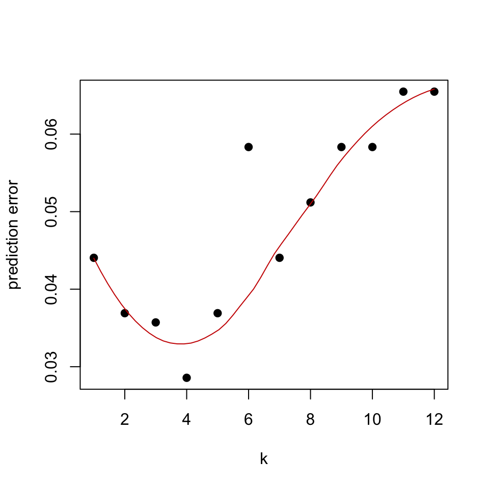

FIGURE 5.8: Cross-validated estimate of prediction error of k in k-NN models.

Based on Figure 5.8 the cross-validation accuracy reveals that \(k=5\) is the best \(k\) value. On the other hand, we can also try bootstrap resampling and check the prediction error that way. We will again use the caret::trainControl() function to do the bootstrap sampling and estimate OOB-based error. However, for a small number of samples like we have in our example, the difference between the estimated and the true value of the prediction error can be large. Below we show how to use bootstrapping for the k-NN model.

set.seed(17)
# this method controls everything about training
# we will just set up 100 bootstrap samples and for each 
# bootstrap OOB samples to test the error
trctrl <- trainControl(method = "boot",number=20,
                       returnResamp="all")

# we will now train k-NN model
knn_fit <- train(subtype~., data = training, 
                 method = "knn",
                 trControl=trctrl,
                 tuneGrid = data.frame(k=1:12))

References

Friedman, Hastie, and Tibshirani. 2001. The Elements of Statistical Learning. Vol. 1. Springer series in statistics New York.