3.1 How to summarize collection of data points: The idea behind statistical distributions
In biology and many other fields, data is collected via experimentation. The nature of the experiments and natural variation in biology makes it impossible to get the same exact measurements every time you measure something. For example, if you are measuring gene expression values for a certain gene, say PAX6, and let’s assume you are measuring expression per sample and cell with any method (microarrays, rt-qPCR, etc.). You will not get the same expression value even if your samples are homogeneous, due to technical bias in experiments or natural variation in the samples. Instead, we would like to describe this collection of data some other way that represents the general properties of the data. Figure 3.1 shows a sample of 20 expression values from the PAX6 gene.
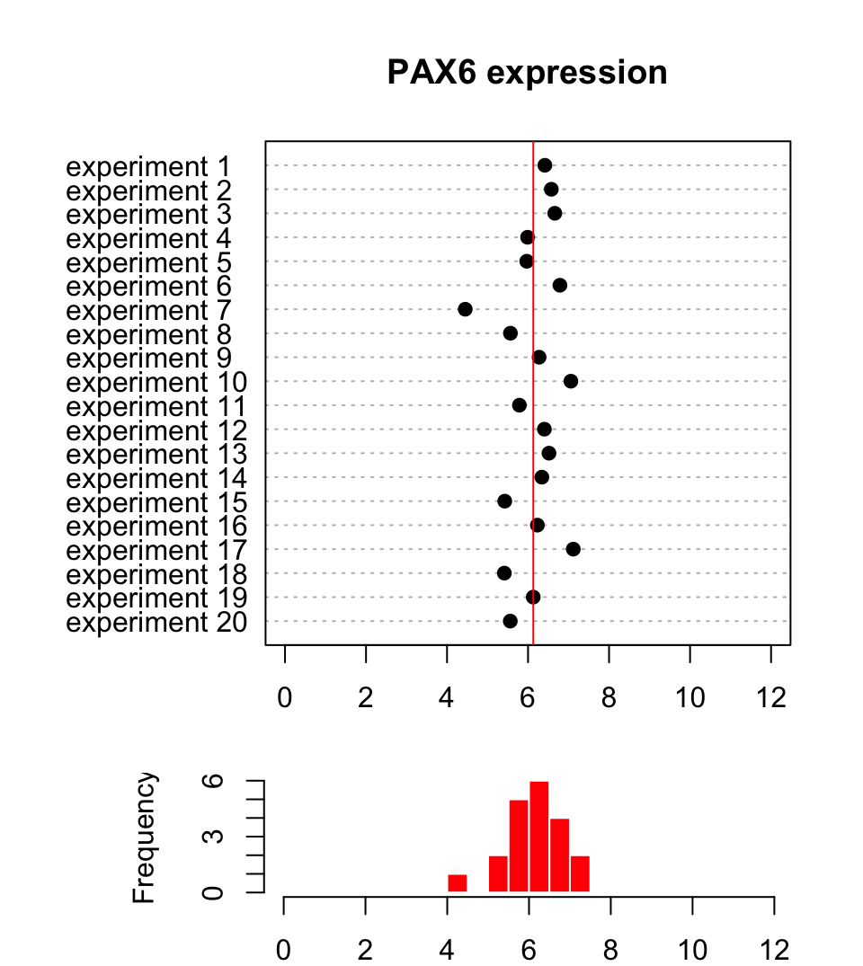
FIGURE 3.1: Expression of the PAX6 gene in 20 replicate experiments.
3.1.1 Describing the central tendency: Mean and median
As seen in Figure 3.1, the points from this sample are distributed around
a central value and the histogram below the dot plot shows the number of points in
each bin. Another observation is that there are some bins that have more points than others. If we want to summarize what we observe, we can try
to represent the collection of data points
with an expression value that is typical to get, something that represents the
general tendency we observe on the dot plot and the histogram. This value is
sometimes called the central
value or central tendency, and there are different ways to calculate such a value.
In Figure 3.1, we see that all the values are spread around 6.13 (red line),
and that is indeed what we call the mean value of this sample of expression values.
It can be calculated with the following formula \(\overline{X}=\sum_{i=1}^n x_i/n\),
where \(x_i\) is the expression value of an experiment and \(n\) is the number of
expression values obtained from the experiments. In R, the mean() function will calculate the
mean of a provided vector of numbers. This is called a “sample mean”. In reality, there are many more than 20 possible PAX6 expression values (provided each cell is of the
identical cell type and is in identical conditions). If we had the time and the funding to sample all cells and measure PAX6 expression we would
get a collection of values that would be called, in statistics, a “population”. In
our case, the population will look like the left hand side of the Figure 3.2. What we have done with
our 20 data points is that we took a sample of PAX6 expression values from this
population, and calculated the sample mean.
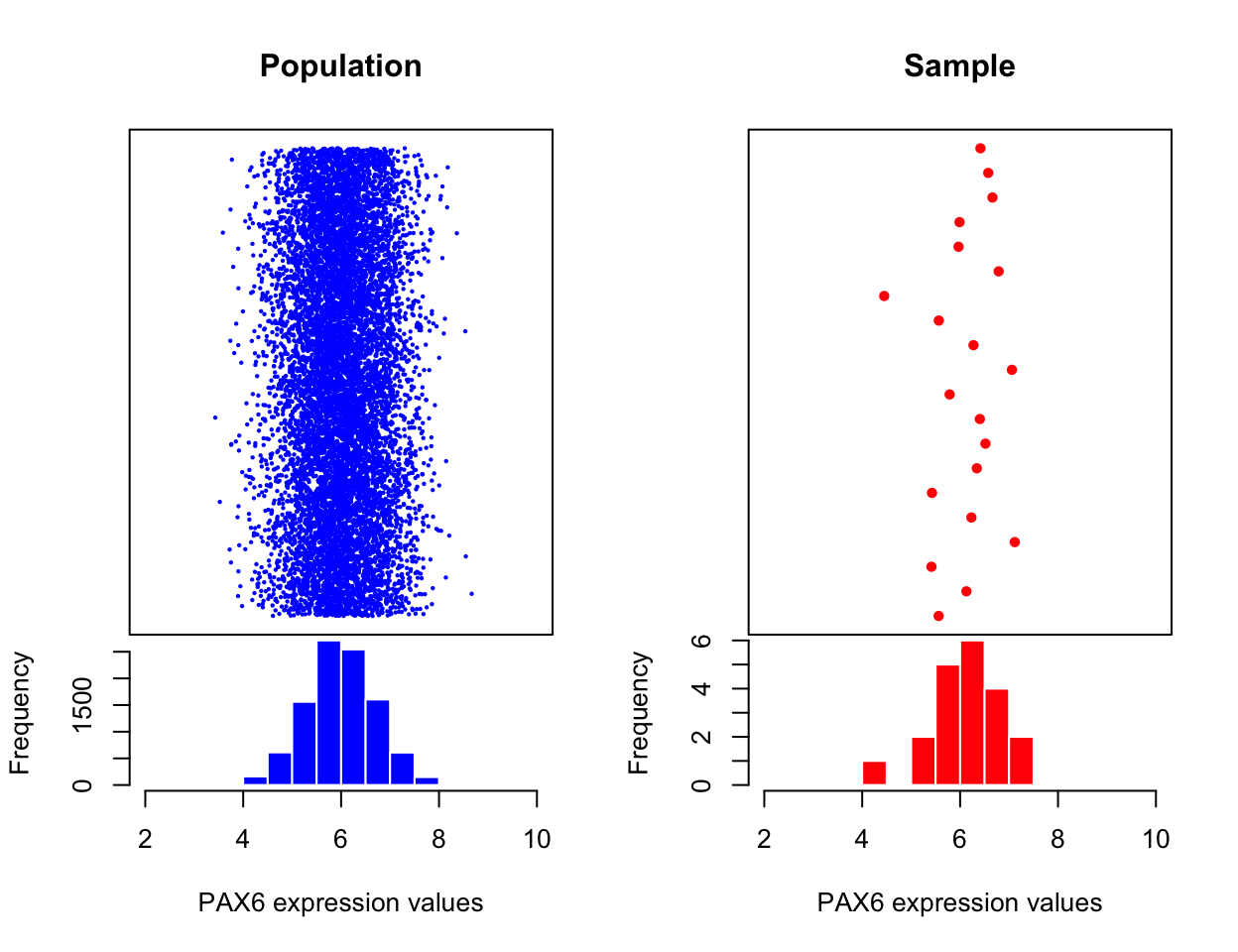
FIGURE 3.2: Expression of all possible PAX6 gene expression measures on all available biological samples (left). Expression of the PAX6 gene from the statistical sample, a random subset from the population of biological samples (right).
The mean of the population is calculated the same way but traditionally the Greek letter \(\mu\) is used to denote the population mean. Normally, we would not have access to the population and we will use the sample mean and other quantities derived from the sample to estimate the population properties. This is the basic idea behind statistical inference, which we will see in action in later sections as well. We estimate the population parameters from the sample parameters and there is some uncertainty associated with those estimates. We will be trying to assess those uncertainties and make decisions in the presence of those uncertainties.
We are not yet done with measuring central tendency.
There are other ways to describe it, such as the median value. The
mean can be affected by outliers easily.
If certain values are very high or low compared to the
bulk of the sample, this will shift mean toward those outliers. However, the median is not affected by outliers. It is simply the value in a distribution where half
of the values are above and the other half are below. In R, the median() function
will calculate the mean of a provided vector of numbers. Let’s create a set of random numbers and calculate their mean and median using
R.
## [1] 0.3738963## [1] 0.32778963.1.2 Describing the spread: Measurements of variation
Another useful way to summarize a collection of data points is to measure
how variable the values are. You can simply describe the range of the values,
such as the minimum and maximum values. You can easily do that in R with the range()
function. A more common way to calculate variation is by calculating something
called “standard deviation” or the related quantity called “variance”. This is a
quantity that shows how variable the values are. A value around zero indicates
there is not much variation in the values of the data points, and a high value
indicates high variation in the values. The variance is the squared distance of
data points from the mean. Population variance is again a quantity we usually
do not have access to and is simply calculated as follows \(\sigma^2=\sum_{i=1}^n \frac{(x_i-\mu)^2}{n}\), where \(\mu\) is the population mean, \(x_i\) is the \(i\)th
data point in the population and \(n\) is the population size. However, when we only have access to a sample, this formulation is biased. That means that it
underestimates the population variance, so we make a small adjustment when we
calculate the sample variance, denoted as \(s^2\):
\[ \begin{aligned} s^2=\sum_{i=1}^n \frac{(x_i-\overline{X})^2}{n-1} && \text{ where $x_i$ is the ith data point and $\overline{X}$ is the sample mean.} \end{aligned} \]
The sample standard deviation is simply the square root of the sample variance, \(s=\sqrt{\sum_{i=1}^n \frac{(x_i-\overline{X})^2}{n-1}}\). The good thing about standard deviation is that it has the same unit as the mean so it is more intuitive.
We can calculate the sample standard deviation and variation with the sd() and var()
functions in R. These functions take a vector of numeric values as input and
calculate the desired quantities. Below we use those functions on a randomly
generated vector of numbers.
## [1] 0.2531495## [1] 0.5031397One potential problem with the variance is that it could be affected by
outliers. The points that are too far away from the mean will have a large
effect on the variance even though there might be few of them.
A way to measure variance that could be less affected by outliers is
looking at where the bulk of the distribution is. How do we define where the bulk is?
One common way is to look at the difference between 75th percentile and 25th
percentile, this effectively removes a lot of potential outliers which will be
towards the edges of the range of values.
This is called the interquartile range, and
can be easily calculated using R via the IQR() function and the quantiles of a vector
are calculated with the quantile() function.
Let us plot the boxplot for a random vector and also calculate IQR using R. In the boxplot (Figure 3.3), 25th and 75th percentiles are the edges of the box, and the median is marked with a thick line cutting through the box.
## [1] 0.5010954## 0% 25% 50% 75% 100%
## 5.437119 5.742895 5.860302 6.243991 6.558112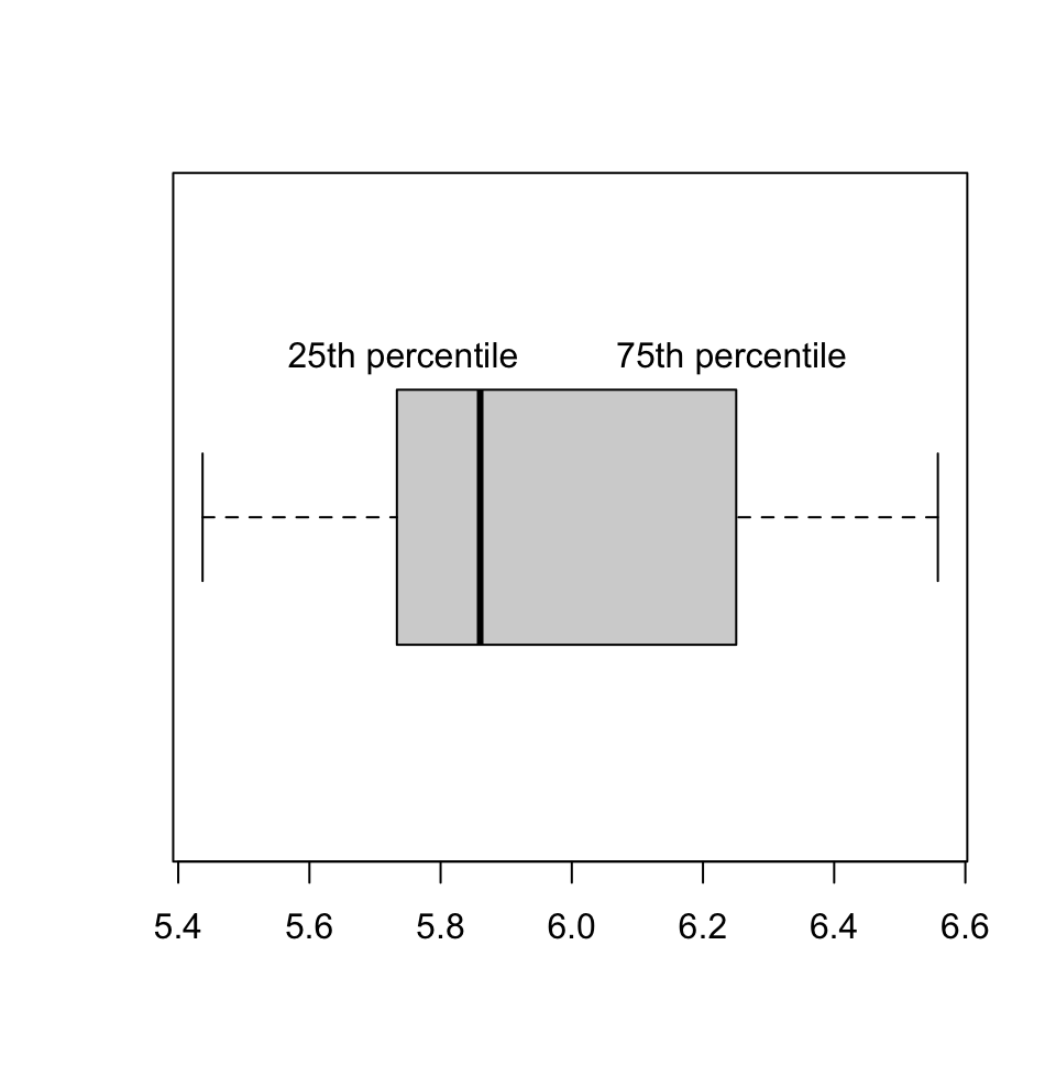
FIGURE 3.3: Boxplot showing the 25th percentile and 75th percentile and median for a set of points sampled from a normal distribution with mean=6 and standard deviation=0.7.
3.1.2.1 Frequently used statistical distributions
The distributions have parameters (such as mean and variance) that summarize them, but also they are functions that assign each outcome of a statistical experiment to its probability of occurrence. One distribution that you will frequently encounter is the normal distribution or Gaussian distribution. The normal distribution has a typical “bell-curve” shape and is characterized by mean and standard deviation. A set of data points that follow normal distribution will mostly be close to the mean but spread around it, controlled by the standard deviation parameter. That means that if we sample data points from a normal distribution, we are more likely to sample data points near the mean and sometimes away from the mean. The probability of an event occurring is higher if it is nearby the mean. The effect of the parameters for the normal distribution can be observed in the following plot.
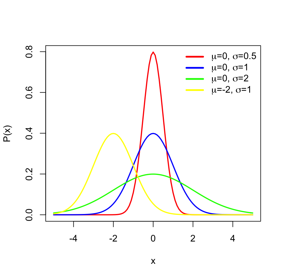
FIGURE 3.4: Different parameters for normal distribution and effect of those on the shape of the distribution
The normal distribution is often denoted by \(\mathcal{N}(\mu,\,\sigma^2)\). When a random variable \(X\) is distributed normally with mean \(\mu\) and variance \(\sigma^2\), we write:
\[X\ \sim\ \mathcal{N}(\mu,\,\sigma^2)\]
The probability density function of the normal distribution with mean \(\mu\) and standard deviation \(\sigma\) is as follows:
\[P(x)=\frac{1}{\sigma\sqrt{2\pi} } \; e^{ -\frac{(x-\mu)^2}{2\sigma^2} } \]
The probability density function gives the probability of observing a value on a normal distribution defined by the \(\mu\) and \(\sigma\) parameters.
Oftentimes, we do not need the exact probability of a value, but we need the probability of observing a value larger or smaller than a critical value or reference point. For example, we might want to know the probability of \(X\) being smaller than or equal to -2 for a normal distribution with mean \(0\) and standard deviation \(2\): \(P(X <= -2 \; | \; \mu=0,\sigma=2)\). In this case, what we want is the area under the curve shaded in dark blue. To be able to do that, we need to integrate the probability density function but we will usually let software do that. Traditionally, one calculates a Z-score which is simply \((X-\mu)/\sigma=(-2-0)/2= -1\), and corresponds to how many standard deviations you are away from the mean. This is also called “standardization”, the corresponding value is distributed in “standard normal distribution” where \(\mathcal{N}(0,\,1)\). After calculating the Z-score, we can look up the area under the curve for the left and right sides of the Z-score in a table, but again, we use software for that. The tables are outdated when you can use a computer.
Below in Figure 3.5, we show the Z-score and the associated probabilities derived from the calculation above for \(P(X <= -2 \; | \; \mu=0,\sigma=2)\).
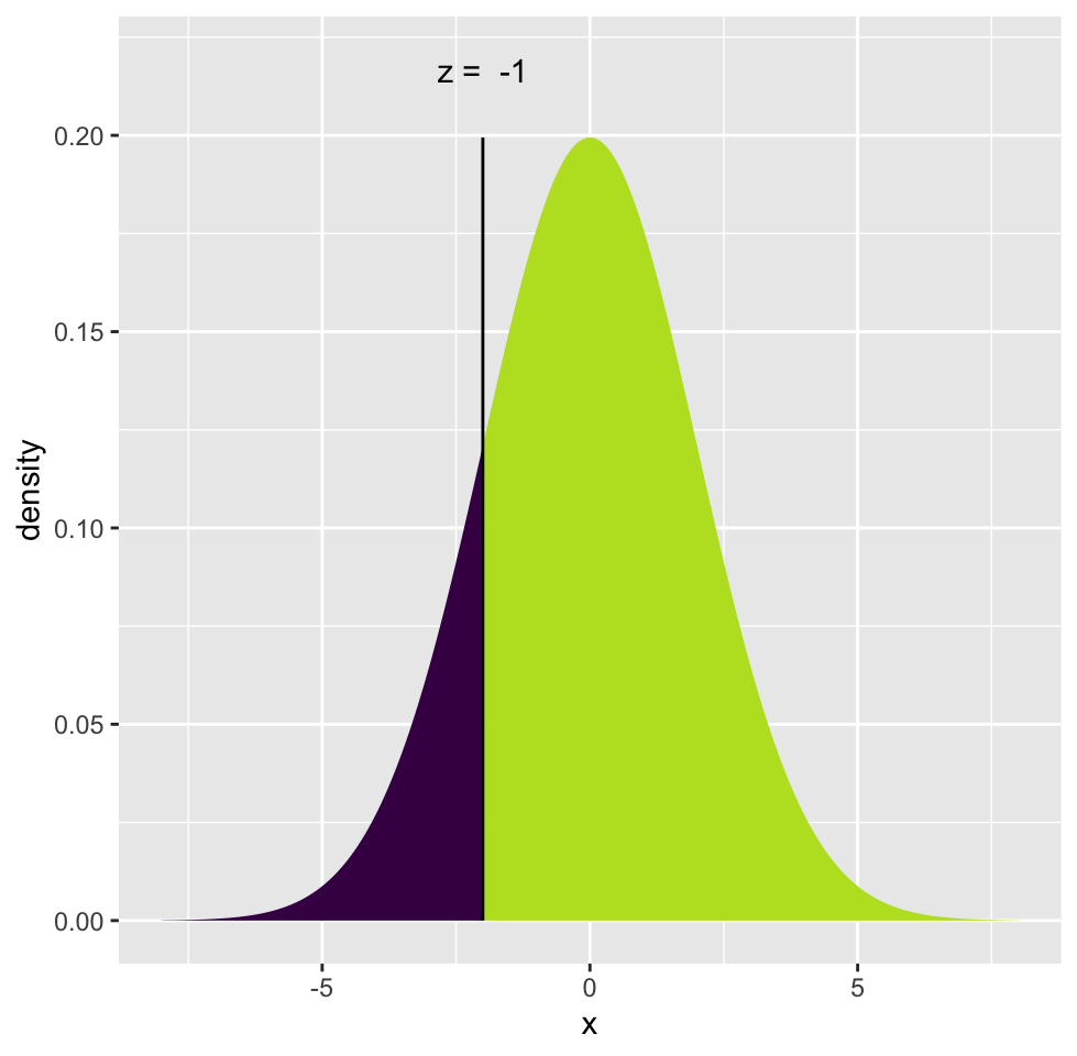
FIGURE 3.5: Z-score and associated probabilities for Z= -1
In R, the family of *norm functions (rnorm,dnorm,qnorm and pnorm) can
be used to
operate with the normal distribution, such as calculating probabilities and
generating random numbers drawn from a normal distribution. We show some of those capabilities below.
# get the value of probability density function when X= -2,
# where mean=0 and sd=2
dnorm(-2, mean=0, sd=2)
## [1] 0.1209854## [1] 0.1586553## [1] 0.8413447## [1] -1.8109030 -1.9220710 -0.5146717 0.8216728 -0.7900804## [1] -2.072867There are many other distribution functions in R that can be used the same way. You have to enter the distribution-specific parameters along with your critical value, quantiles, or number of random numbers depending on which function you are using in the family. We will list some of those functions below.
dbinomis for the binomial distribution. This distribution is usually used to model fractional data and binary data. Examples from genomics include methylation data.dpoisis used for the Poisson distribution anddnbinomis used for the negative binomial distribution. These distributions are used to model count data such as sequencing read counts.df(F distribution) anddchisq(Chi-Squared distribution) are used in relation to the distribution of variation. The F distribution is used to model ratios of variation and Chi-Squared distribution is used to model distribution of variations. You will frequently encounter these in linear models and generalized linear models.
3.1.3 Precision of estimates: Confidence intervals
When we take a random sample from a population and compute a statistic, such as the mean, we are trying to approximate the mean of the population. How well this sample statistic estimates the population value will always be a concern. A confidence interval addresses this concern because it provides a range of values which will plausibly contain the population parameter of interest. Normally, we would not have access to a population. If we did, we would not have to estimate the population parameters and their precision.
When we do not have access to the population, one way to estimate intervals is to repeatedly take samples from the original sample with replacement, that is, we take a data point from the sample we replace, and we take another data point until we have sample size of the original sample. Then, we calculate the parameter of interest, in this case the mean, and repeat this process a large number of times, such as 1000. At this point, we would have a distribution of re-sampled means. We can then calculate the 2.5th and 97.5th percentiles and these will be our so-called 95% confidence interval. This procedure, resampling with replacement to estimate the precision of population parameter estimates, is known as the bootstrap resampling or bootstraping.
Let’s see how we can do this in practice. We simulate a sample coming from a normal distribution (but we pretend we don’t know the population parameters). We will estimate the precision of the mean of the sample using bootstrapping to build confidence intervals, the resulting plot after this procedure is shown in Figure 3.6.
library(mosaic)
set.seed(21)
sample1= rnorm(50,20,5) # simulate a sample

# do bootstrap resampling, sampling with replacement
boot.means=do(1000) * mean(resample(sample1))

# get percentiles from the bootstrap means
q=quantile(boot.means[,1],p=c(0.025,0.975))

# plot the histogram
hist(boot.means[,1],col="cornflowerblue",border="white",
                    xlab="sample means")
abline(v=c(q[1], q[2] ),col="red")
text(x=q[1],y=200,round(q[1],3),adj=c(1,0))
text(x=q[2],y=200,round(q[2],3),adj=c(0,0))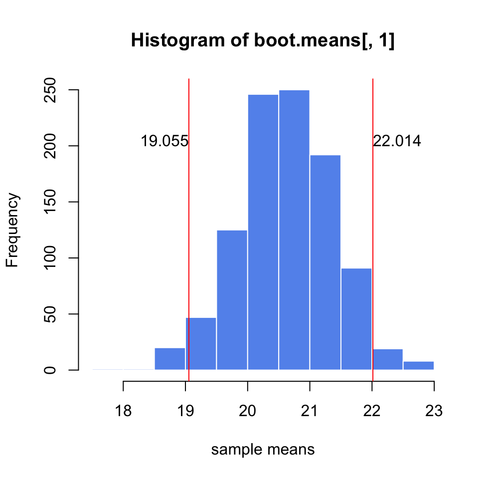
FIGURE 3.6: Precision estimate of the sample mean using 1000 bootstrap samples. Confidence intervals derived from the bootstrap samples are shown with red lines.
If we had a convenient mathematical method to calculate the confidence interval, we could also do without resampling methods. It turns out that if we take repeated samples from a population with sample size \(n\), the distribution of means (\(\overline{X}\)) of those samples will be approximately normal with mean \(\mu\) and standard deviation \(\sigma/\sqrt{n}\). This is also known as the Central Limit Theorem(CLT) and is one of the most important theorems in statistics. This also means that \(\frac{\overline{X}-\mu}{\sigma\sqrt{n}}\) has a standard normal distribution and we can calculate the Z-score, and then we can get the percentiles associated with the Z-score. Below, we are showing the Z-score calculation for the distribution of \(\overline{X}\), and then we are deriving the confidence intervals starting with the fact that the probability of Z being between \(-1.96\) and \(1.96\) is \(0.95\). We then use algebra to show that the probability that unknown \(\mu\) is captured between \(\overline{X}-1.96\sigma/\sqrt{n}\) and \(\overline{X}+1.96\sigma/\sqrt{n}\) is \(0.95\), which is commonly known as the 95% confidence interval.
\[\begin{array}{ccc} Z=\frac{\overline{X}-\mu}{\sigma/\sqrt{n}}\\ P(-1.96 < Z < 1.96)=0.95 \\ P(-1.96 < \frac{\overline{X}-\mu}{\sigma/\sqrt{n}} < 1.96)=0.95\\ P(\mu-1.96\sigma/\sqrt{n} < \overline{X} < \mu+1.96\sigma/\sqrt{n})=0.95\\ P(\overline{X}-1.96\sigma/\sqrt{n} < \mu < \overline{X}+1.96\sigma/\sqrt{n})=0.95\\ confint=[\overline{X}-1.96\sigma/\sqrt{n},\overline{X}+1.96\sigma/\sqrt{n}] \end{array}\]
A 95% confidence interval for the population mean is the most common interval to use, and would mean that we would expect 95% of the interval estimates to include the population parameter, in this case, the mean. However, we can pick any value such as 99% or 90%. We can generalize the confidence interval for \(100(1-\alpha)\) as follows:
\[\overline{X} \pm Z_{\alpha/2}\sigma/\sqrt{n}\]
In R, we can do this using the qnorm() function to get Z-scores associated
with \({\alpha/2}\) and \({1-\alpha/2}\). As you can see, the confidence intervals we calculated using CLT are very
similar to the ones we got from the bootstrap for the same sample. For bootstrap we got \([19.21, 21.989]\) and for the CLT-based estimate we got \([19.23638, 22.00819]\).
## [1] 19.23638 22.00819The good thing about CLT is, as long as the sample size is large, regardless of the population distribution, the distribution of sample means drawn from that population will always be normal. In Figure 3.7, we repeatedly draw samples 1000 times with sample size \(n=10\),\(30\), and \(100\) from a bimodal, exponential and a uniform distribution and we are getting sample mean distributions following normal distribution.
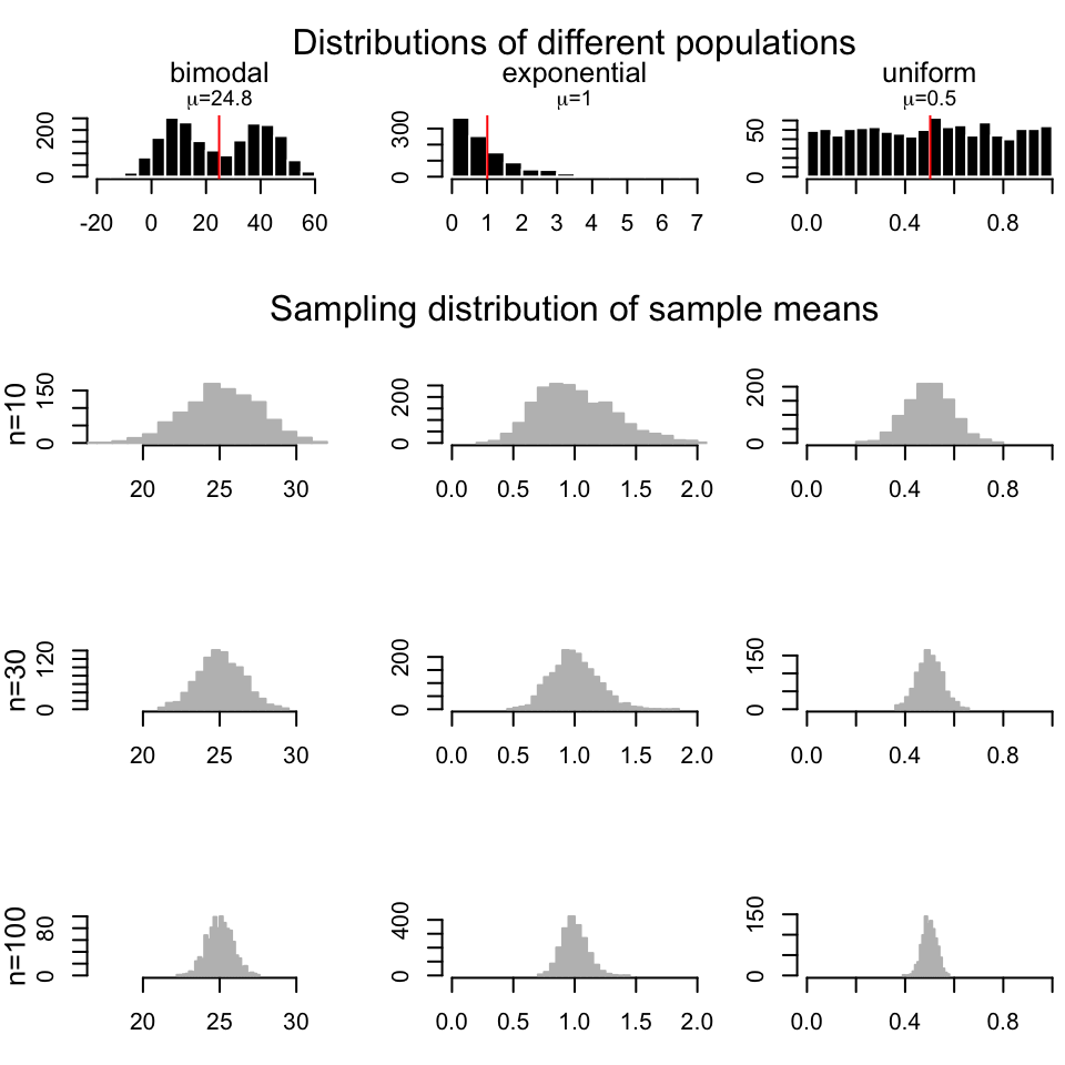
FIGURE 3.7: Sample means are normally distributed regardless of the population distribution they are drawn from.
However, we should note that how we constructed the confidence interval using standard normal distribution, \(N(0,1)\), only works when we know the population standard deviation. In reality, we usually have only access to a sample and have no idea about the population standard deviation. If this is the case, we should estimate the standard deviation using the sample standard deviation and use something called the t distribution instead of the standard normal distribution in our interval calculation. Our confidence interval becomes \(\overline{X} \pm t_{\alpha/2}s/\sqrt{n}\), with t distribution parameter \(d.f=n-1\), since now the following quantity is t distributed \(\frac{\overline{X}-\mu}{s/\sqrt{n}}\) instead of standard normal distribution.
The t distribution is similar to the standard normal distribution and has mean \(0\) but its spread is larger than the normal distribution especially when the sample size is small, and has one parameter \(v\) for the degrees of freedom, which is \(n-1\) in this case. Degrees of freedom is simply the number of data points minus the number of parameters estimated.Here we are estimating the mean from the data, therefore the degrees of freedom is \(n-1\). The resulting distributions are shown in Figure 3.8.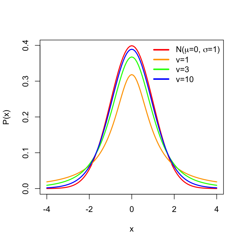
FIGURE 3.8: Normal distribution and t distribution with different degrees of freedom. With increasing degrees of freedom, the t distribution approximates the normal distribution better.