6.3 Dealing with continuous scores over the genome
Most high-throughput data can be viewed as a continuous score over the bases of the genome. In case of RNA-seq or ChIP-seq experiments, the data can be represented as read coverage values per genomic base position. In addition, other information (not necessarily from high-throughput experiments) can be represented this way. The GC content and conservation scores per base are prime examples of other data sets that can be represented as scores over the genome. This sort of data can be stored as a generic text file or can have special formats such as Wig (stands for wiggle) from UCSC, or the bigWig format, which is an indexed binary format of the wig files. The bigWig format is great for data that covers a large fraction of the genome with varying scores, because the file is much smaller than regular text files that have the same information and it can be queried more easily since it is indexed.
In R/Bioconductor, continuous data can also be represented in a compressed format, called Rle vector, which stands for run-length encoded vector. This gives superior memory performance over regular vectors because repeating consecutive values are represented as one value in the Rle vector (see Figure 6.3).
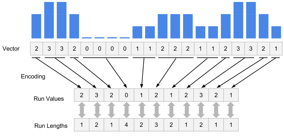
FIGURE 6.3: Rle encoding explained.
Typically, for genome-wide data you will have an RleList object, which is a list of Rle vectors per chromosome. You can obtain such vectors by reading the reads in and calling the coverage() function from the GenomicRanges package. Let’s try that on the above data set.
## RleList of length 24
## $chr1
## integer-Rle of length 249250621 with 1 run
##   Lengths: 249250621
##   Values :         0
##
## $chr2
## integer-Rle of length 243199373 with 1 run
##   Lengths: 243199373
##   Values :         0
##
## $chr3
## integer-Rle of length 198022430 with 1 run
##   Lengths: 198022430
##   Values :         0
##
## $chr4
## integer-Rle of length 191154276 with 1 run
##   Lengths: 191154276
##   Values :         0
##
## $chr5
## integer-Rle of length 180915260 with 1 run
##   Lengths: 180915260
##   Values :         0
##
## ...
## <19 more elements>
Alternatively, you can get the coverage from the BAM file directly. Below, we are getting the coverage directly from the BAM file for our previously defined promoters.
One of the most common ways of storing score data is, as mentioned, the wig or bigWig format. Most of the ENCODE project data can be downloaded in bigWig format. In addition, conservation scores can also be downloaded in the wig/bigWig format. You can import bigWig files into R using the import() function from the rtracklayer package. However, it is generally not advisable to read the whole bigWig file in memory as was the case with BAM files. Usually, you will be interested in only a fraction of the genome, such as promoters, exons etc. So it is best that you extract the data for those regions and read those into memory rather than the whole file. Below we read a bigWig file only for the bases on promoters. The operation returns a GRanges object with the score column which indicates the scores in the bigWig file per genomic region.
library(rtracklayer)

# File from ENCODE ChIP-seq tracks
bwFile=system.file("extdata",
                      "wgEncodeHaibTfbsA549.chr21.bw",
                      package="compGenomRData")
bw.gr=import(bwFile, which=promoter.gr) # get coverage vectors
bw.gr
## GRanges object with 9205 ranges and 1 metadata column:
## seqnames ranges strand | score
## <Rle> <IRanges> <Rle> | <numeric>
## [1] chr21 9825456-9825457 * | 1
## [2] chr21 9825458-9825464 * | 2
## [3] chr21 9825465-9825466 * | 4
## [4] chr21 9825467-9825470 * | 5
## [5] chr21 9825471 * | 6
## ... ... ... ... . ...
## [9201] chr21 48055809-48055856 * | 2
## [9202] chr21 48055857-48055858 * | 1
## [9203] chr21 48055872-48055921 * | 1
## [9204] chr21 48055944-48055993 * | 1
## [9205] chr21 48056069-48056118 * | 1
## -------
## seqinfo: 1 sequence from an unspecified genomeFollowing this we can create an RleList object from the GRanges with the coverage() function.
cov.bw=coverage(bw.gr,weight = "score")

# or get this directly from
cov.bw=import(bwFile, which=promoter.gr,as = "RleList")
6.3.1 Extracting subsections of Rle and RleList objects
Frequently, we will need to extract subsections of the Rle vectors or RleList objects.
We will need to do this to visualize that subsection or get some statistics out
of those sections. For example, we could be interested in average coverage per
base for the regions we are interested in. We have to extract those regions
from the RleList object and apply summary statistics. Below, we show how to extract
subsections of the RleList object. We are extracting promoter regions from the ChIP-seq
read coverage RleList. Following that, we will plot one of the promoter’s coverage values.
myViews=Views(cov.bw,as(promoter.gr,"IRangesList")) # get subsets of coverage
# there is a views object for each chromosome
myViews
## RleViewsList object of length 1:
## $chr21
## Views on a 48129895-length Rle subject
##
## views:
##          start      end width
##   [1] 42218039 42220039  2001 [2 0 0 0 0 0 0 0 0 0 0 0 0 0 0 0 0 0 0 0 0 ...]
##   [2] 17441841 17443841  2001 [0 0 0 0 0 0 0 0 0 0 0 0 0 0 0 0 0 0 0 0 0 ...]
##   [3] 17565698 17567698  2001 [0 0 0 0 0 0 0 0 0 0 0 0 0 0 0 0 0 0 0 0 0 ...]
##   [4] 30395937 30397937  2001 [0 0 0 0 0 0 0 0 0 0 0 0 0 0 0 0 0 0 0 0 0 ...]
##   [5] 27542138 27544138  2001 [1 1 1 1 1 1 1 1 1 1 1 1 1 2 2 2 2 2 1 1 1 ...]
##   [6] 27511708 27513708  2001 [0 0 0 0 0 0 0 0 0 0 0 0 0 0 0 0 0 0 0 0 0 ...]
##   [7] 32930290 32932290  2001 [0 0 0 0 0 0 0 0 0 0 0 0 0 0 0 0 0 0 0 0 0 ...]
##   [8] 27542446 27544446  2001 [0 0 0 0 0 0 0 0 0 0 0 0 0 0 0 0 0 0 0 0 0 ...]
##   [9] 28338439 28340439  2001 [0 0 0 0 0 0 0 0 0 0 0 0 0 0 0 0 0 0 0 0 0 ...]
##   ...      ...      ...   ... ...
## [370] 47517032 47519032  2001 [1 1 1 1 1 1 1 1 1 1 1 1 1 1 1 1 1 1 1 1 1 ...]
## [371] 47648157 47650157  2001 [1 1 1 1 1 1 1 1 1 1 1 1 1 1 1 1 1 1 1 1 1 ...]
## [372] 47603373 47605373  2001 [0 0 0 0 0 0 0 0 0 0 0 0 0 0 0 0 0 0 0 0 0 ...]
## [373] 47647738 47649738  2001 [2 2 2 2 2 2 2 2 2 2 2 2 2 2 2 2 2 2 2 1 2 ...]
## [374] 47704236 47706236  2001 [0 0 0 0 0 0 0 0 0 0 0 0 0 0 0 0 0 0 0 0 0 ...]
## [375] 47742785 47744785  2001 [0 0 0 0 0 0 0 0 0 0 0 0 0 0 0 0 0 0 0 0 0 ...]
## [376] 47881383 47883383  2001 [1 1 1 1 1 1 1 1 1 1 1 1 1 1 1 1 1 1 1 1 1 ...]
## [377] 48054506 48056506  2001 [0 0 0 0 0 0 0 0 0 0 0 0 0 0 0 0 0 0 0 0 0 ...]
## [378] 48024035 48026035 2001 [1 1 1 1 1 1 1 1 1 1 1 1 1 1 1 1 1 1 1 1 1 ...]## Views on a 48129895-length Rle subject
##
## views:
## start end width
## [1] 42218039 42220039 2001 [2 0 0 0 0 0 0 0 0 0 0 0 0 0 0 0 0 0 0 0 0 ...]
## [2] 17441841 17443841 2001 [0 0 0 0 0 0 0 0 0 0 0 0 0 0 0 0 0 0 0 0 0 ...]
## [3] 17565698 17567698 2001 [0 0 0 0 0 0 0 0 0 0 0 0 0 0 0 0 0 0 0 0 0 ...]
## [4] 30395937 30397937 2001 [0 0 0 0 0 0 0 0 0 0 0 0 0 0 0 0 0 0 0 0 0 ...]
## [5] 27542138 27544138 2001 [1 1 1 1 1 1 1 1 1 1 1 1 1 2 2 2 2 2 1 1 1 ...]
## [6] 27511708 27513708 2001 [0 0 0 0 0 0 0 0 0 0 0 0 0 0 0 0 0 0 0 0 0 ...]
## [7] 32930290 32932290 2001 [0 0 0 0 0 0 0 0 0 0 0 0 0 0 0 0 0 0 0 0 0 ...]
## [8] 27542446 27544446 2001 [0 0 0 0 0 0 0 0 0 0 0 0 0 0 0 0 0 0 0 0 0 ...]
## [9] 28338439 28340439 2001 [0 0 0 0 0 0 0 0 0 0 0 0 0 0 0 0 0 0 0 0 0 ...]
## ... ... ... ... ...
## [370] 47517032 47519032 2001 [1 1 1 1 1 1 1 1 1 1 1 1 1 1 1 1 1 1 1 1 1 ...]
## [371] 47648157 47650157 2001 [1 1 1 1 1 1 1 1 1 1 1 1 1 1 1 1 1 1 1 1 1 ...]
## [372] 47603373 47605373 2001 [0 0 0 0 0 0 0 0 0 0 0 0 0 0 0 0 0 0 0 0 0 ...]
## [373] 47647738 47649738 2001 [2 2 2 2 2 2 2 2 2 2 2 2 2 2 2 2 2 2 2 1 2 ...]
## [374] 47704236 47706236 2001 [0 0 0 0 0 0 0 0 0 0 0 0 0 0 0 0 0 0 0 0 0 ...]
## [375] 47742785 47744785 2001 [0 0 0 0 0 0 0 0 0 0 0 0 0 0 0 0 0 0 0 0 0 ...]
## [376] 47881383 47883383 2001 [1 1 1 1 1 1 1 1 1 1 1 1 1 1 1 1 1 1 1 1 1 ...]
## [377] 48054506 48056506 2001 [0 0 0 0 0 0 0 0 0 0 0 0 0 0 0 0 0 0 0 0 0 ...]
## [378] 48024035 48026035 2001 [1 1 1 1 1 1 1 1 1 1 1 1 1 1 1 1 1 1 1 1 1 ...]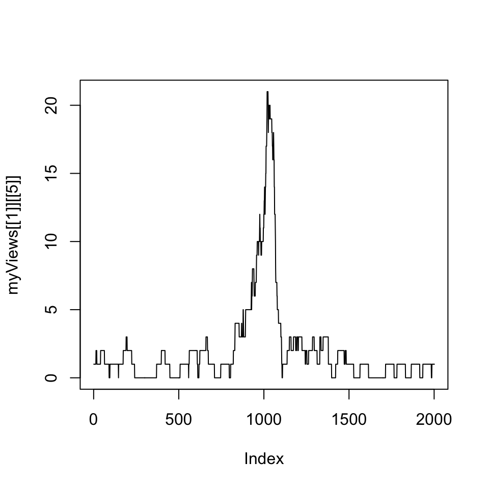
FIGURE 6.4: Coverage vector extracted from the RleList via the Views() function is plotted as a line plot.
Next, we are interested in average coverage per base for the promoters using summary
functions that work on the Views object.
## [1] 0.2258871 0.3498251 1.2243878 0.4997501 2.0904548 0.6996502## [1] 2 4 12 4 21 6