9.7 Motif discovery
The first analysis step downstream of peak calling is motif discovery. Motif discovery is a procedure of finding enriched sets of similar short sequences in a large sequence dataset. In our case the large sequence dataset are sequences around ChIP peaks, while the short sequence sets are the transcription factor binding sites.
There are two types of motif discovery tools: supervised and unsupervised. Supervised tools require explicit positive (we are certain that the motif is enriched), and negative sequence sets (we are certain that the motif is not enriched), and then search for relative enrichment of short motifs in the foreground versus the background. Unsupervised models, on the other hand, require only a set of positive sequences, and then compare motif abundance to a statistically constructed background set.
Due to the combinatorial nature of the procedure, motif discovery is
computationally expensive. It is therefore often performed on a subset of the
highest-quality peaks. In this tutorial we will use the rGADEM
package for motif discovery.
rGADEM is an unsupervised, stochastic motif discovery tools, which uses
sampling with subsequent enrichment analysis to find over-represented sequence
motifs.
We will firstly load our CTCF peaks, and convert them to a GRanges object.
We will then select the top 500 peaks, and extract the DNA sequence, which
will be used as input for the motif discovery. Nearby ChIP peaks can have overlapping coordinates. After selection, overlapping CTCF peaks have to be merged using the reduce() function from the GenomicRanges package. If we do not execute this step, we will include the same sequence multiple times in the sequence set, and artificially enrich DNA patterns.
# read the CTCF peaks created in the peak calling part of the tutorial
ctcf_peaks = read.table(file.path(data_path, 'CTCF_peaks.txt'), header=TRUE)

# convert the peaks into a GRanges object
ctcf_peaks = makeGRangesFromDataFrame(ctcf_peaks, keep.extra.columns = TRUE)

# order the peaks by qvalue, and take top 250 peaks
ctcf_peaks = ctcf_peaks[order(ctcf_peaks$qvalue)]
ctcf_peaks = head(ctcf_peaks, n = 500)

# merge nearby CTCF peaks
ctcf_peaks = reduce(ctcf_peaks)
Create a region of \(+/-\) 50 bp around the center of the peaks,
and extract the genomic sequence.
We are now ready to run the motif discovery. Firstly we load the rGADEM package:
To run the motif discovery, we call the GADEM() function. with the
extracted DNA sequences. In addition to the DNA sequences, we need to
specify two parameters:
- seed - the random number generator seed, which will make the analysis reproducible.
- nmotifs - the number of motifs to look for.
## top 3  4, 5-mers: 12 40 52
## top 3  4, 5-mers: 12 36 42
The rGADEM package contains a convenient plot() function for
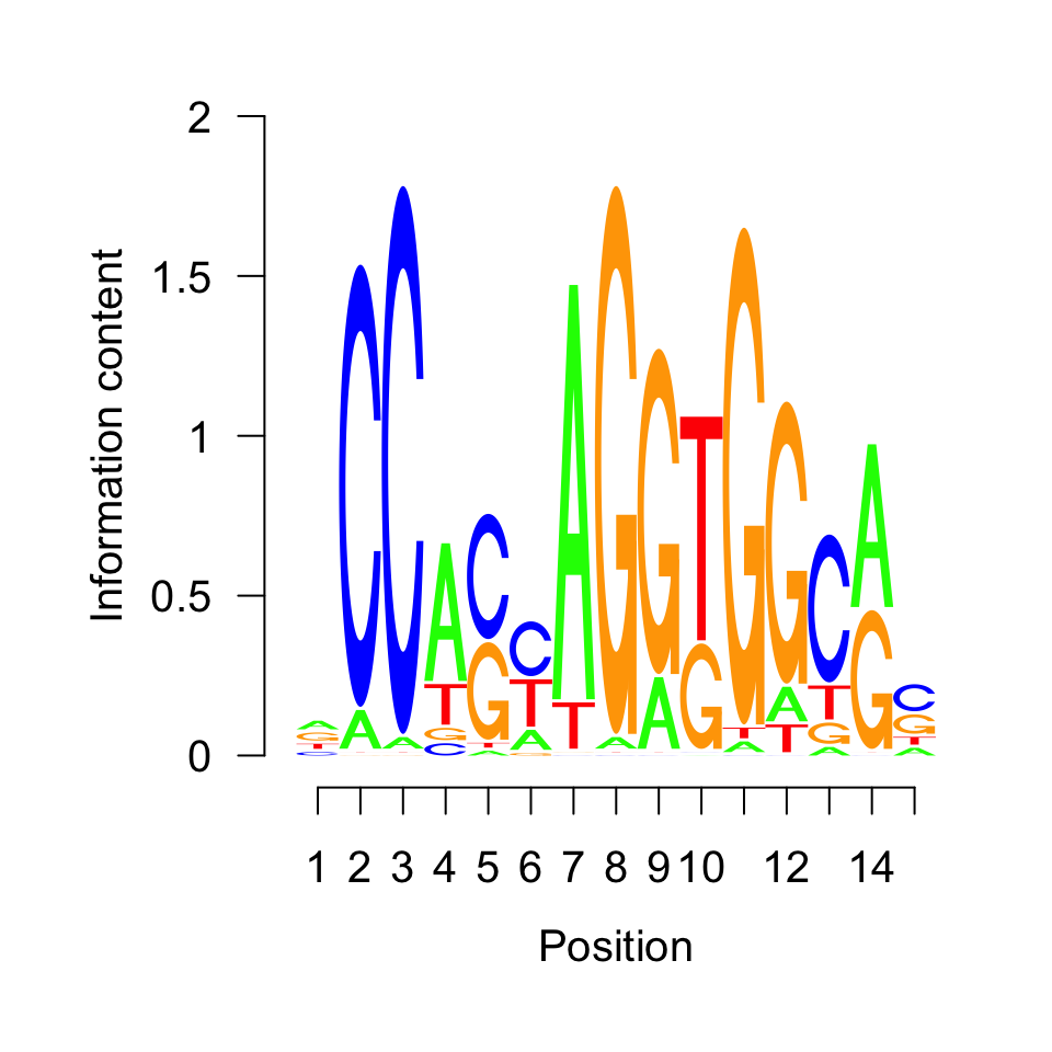
motif visualization. We will use the plot function to visualize the most enriched DNA motif:

FIGURE 9.22: Motif with highest enrichment in top 500 CTCF peaks.
The motif shown in Figure 9.22 corresponds to the previously visualized CTCF motif. Nevertheless, we will computationally annotate our motif by querying the JASPAR (Khan, Fornes, Stigliani, et al. 2018) database in the next section.
9.7.1 Motif comparison
We will now compare our unknown motif with the JASPAR2018 (Khan, Fornes, Stigliani, et al. 2018) database,
to figure out to which transcription factor it corresponds.
Firstly we convert the frequency matrix into a PWMatrix object, and
then use this object to query the database.
# load the TFBSTools library
library(TFBSTools)

# extract the motif of interest from the GADEM object
unknown_motif = getPWM(novel_motifs)[[1]]

# convert the motif to a PWM matrix
unknown_pwm   = PWMatrix(
    ID = 'unknown',
    profileMatrix = unknown_motif
)
Using the getMatrixSet() function we extract all motifs which
correspond to known human transcription factors.
The opts parameter defines which PWM database to use for comparison.
# load the JASPAR motif database
library(JASPAR2018)

# extract motifs corresponding to human transcription factors
pwm_library = getMatrixSet(
  JASPAR2018,
  opts=list(
    collection = 'CORE',
    species    = 'Homo sapiens',
    matrixtype = 'PWM'
  ))
The PWMSimilarity() function calculates the Pearson correlation between
the database, and our discovered motif via rGADEM.
# find the most similar motif to our motif
pwm_sim = PWMSimilarity(

  # JASPAR library
  pwm_library,

  # out motif
  unknown_pwm,

  # measure for comparison
  method = 'Pearson')
We extract the motif names from the PWM library. For each motif in the library we append the Pearson correlation with our unknown motif, and look at the topmost candidates.
# extract the motif names from the pwm library
pwm_library_list = lapply(pwm_library, function(x){
  data.frame(ID = ID(x), name = name(x))
})

# combine the list into one data frame
pwm_library_dt = dplyr::bind_rows(pwm_library_list)

# fetch the similarity of each motif to our unknown motif
pwm_library_dt$similarity = pwm_sim[pwm_library_dt$ID]

# find the most similar motif in the library
pwm_library_dt = pwm_library_dt[order(-pwm_library_dt$similarity),]## ID name similarity
## 24 MA0139.1 CTCF 0.7033789
## 370 MA1100.1 ASCL1 0.4769023
## 281 MA0807.1 TBX5 0.4762250
## 101 MA0033.2 FOXL1 0.4605249
## 302 MA0825.1 MNT 0.4370585
## 277 MA0803.1 TBX15 0.4317270As expected, the topmost candidate is CTCF.
References
Khan, Fornes, Stigliani, et al. 2018. “JASPAR 2018: Update of the Open-Access Database of Transcription Factor Binding Profiles and Its Web Framework.” Nucleic Acids Res 46 (D1): D260–D266. https://doi.org/10.1093/nar/gkx1126.