5.4 Data preprocessing

We will have to preprocess the data before we start training. This might include exploratory data analysis to see how variables and samples relate to each other. For example, we might want to check the correlation between predictor variables and keep only one variable from that group. In addition, some training algorithms might be sensitive to data scales or outliers. We should deal with those issues in this step. In some cases, the data might have missing values. We can choose to remove the samples that have missing values or try to impute them. Many machine learning algorithms will not be able to deal with missing values.

We will show how to do this in practice using the caret::preProcess() function and base R functions. Please note that there are more preprocessing options available than we will show here. There are more possibilities in caret::preProcess()function and base R functions, we are just going to cover a few basics in this section.

5.4.1 Data transformation

The first thing we will do is data normalization and transformation. We have to take care of data scale issues that might come from how the experiments are performed and the potential problems that might occur during data collection. Ideally, each tumor sample has a similar distribution of gene expression values. Systematic differences between tumor samples must be corrected. We check if there are such differences using box plots. We will only plot the first 50 tumor samples so that the figure is not too squished. The resulting boxplot is shown in Figure 5.1.

boxplot(gexp[,1:50],outline=FALSE,col="cornflowerblue")

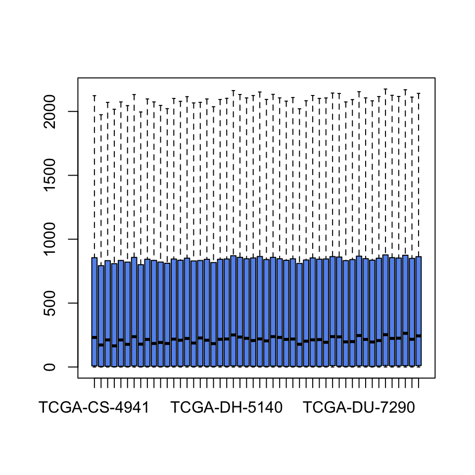
FIGURE 5.1: Boxplots for gene expression values.

It seems there was some normalization done on this data. Gene expression values per sample seem to have the same scale. However, it looks like they have long-tailed distributions, so a log transformation may fix that. These long-tailed distributions have outliers and this might adversely affect the models. Below, we show the effect of log transformation on the gene expression profile of a patient. We add a pseudo count of 1 to avoid log(0). The resulting histograms are shown in Figure 5.2.

par(mfrow=c(1,2))
hist(gexp[,5],xlab="gene expression",main="",border="blue4",
     col="cornflowerblue")
hist(log10(gexp+1)[,5], xlab="gene expression log scale",main="",
     border="blue4",col="cornflowerblue")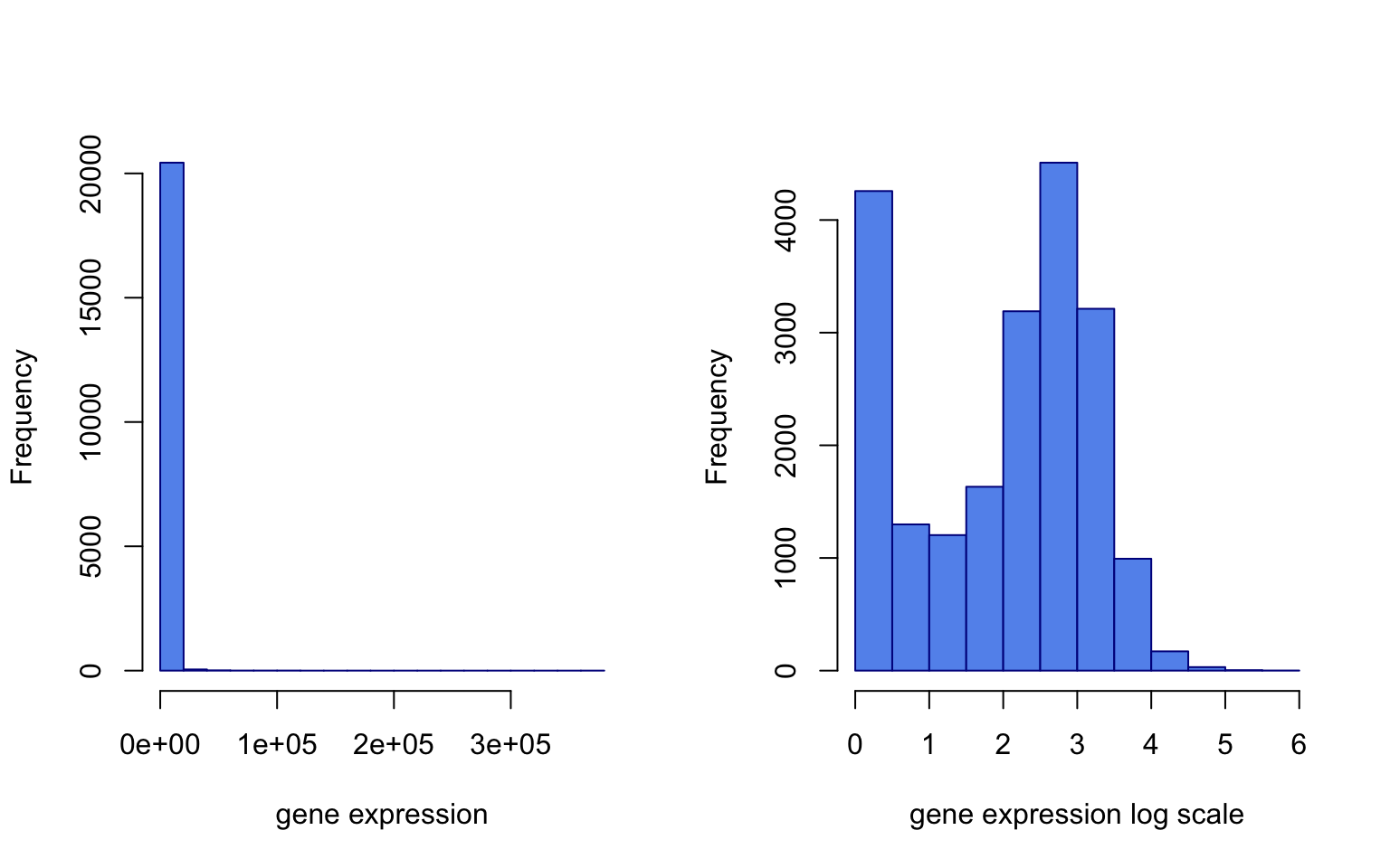

FIGURE 5.2: Gene expression distribution for the 5th patient (left). Log transformed gene expression distribution for the same patient (right).

Since taking a log seems to work to tame the extreme values, we do that below and also add \(1\) pseudo-count to be able to deal with \(0\) values:

gexp=log10(gexp+1)

Another thing we can do in combination with this is to winsorize the data, which caps extreme values to the 1st and 99th percentiles or to other user-defined percentiles. But before we go forward, we should transpose our data. In this case, the predictor variables are gene expression values and they should be on the column side. It was OK to leave them on the row side, to check systematic errors with box plots, but machine learning algorithms require that predictor variables are on the column side.

# transpose the data set
tgexp <- t(gexp)

5.4.2 Filtering data and scaling

We can filter predictor variables which have low variation. They are not likely to have any predictive importance since there is not much variation and they will just slow our algorithms. The more variables, the slower the algorithms will be generally. The caret::preProcess() function can help filter the predictor variables with near zero variance.

library(caret)
# remove near zero variation for the columns at least
# 85% of the values are the same
# this function creates the filter but doesn't apply it yet
nzv=preProcess(tgexp,method="nzv",uniqueCut = 15)

# apply the filter using "predict" function
# return the filtered dataset and assign it to nzv_tgexp
# variable
nzv_tgexp=predict(nzv,tgexp)

In addition, we can also choose arbitrary cutoffs for variability. For example, we can choose to take the top 1000 variable predictors.

SDs=apply(tgexp,2,sd )
topPreds=order(SDs,decreasing = TRUE)[1:1000]
tgexp=tgexp[,topPreds]

We can also center the data, which as we have seen in Chapter 4, is subtracting the mean. Following this, the predictor variables will have zero means. In addition, we can scale the data. When we scale, each value of the predictor variable is divided by its standard deviation. Therefore predictor variables will have the same standard deviation. These manipulations are generally used to improve the numerical stability of some calculations. In distance-based metrics, it could be beneficial to at least center the data. We will now center the data using the preProcess() function. This is more practical than the scale() function because when we get a new data point, we can use the predict() function and processCenter object to process it just like we did for the training samples.

library(caret)
processCenter=preProcess(tgexp, method = c("center"))
tgexp=predict(processCenter,tgexp)

We will next filter the predictor variables that are highly correlated. You may choose not to do this as some methods can handle correlation between predictor variables. However, the fewer predictor variables we have, the faster the model fitting can be done.

# create a filter for removing higly correlated variables
# if two variables are highly correlated only one of them
# is removed
corrFilt=preProcess(tgexp, method = "corr",cutoff = 0.9)
tgexp=predict(corrFilt,tgexp)

5.4.3 Dealing with missing values

In real-life situations, there will be missing values in our data. In genomics, we might not have values for certain genes or genomic locations due to technical problems during experiments. We have to be able to deal with these missing values. For demonstration purposes, we will now introduce NA values in our data, the “NA” value is normally used to encode missing values in R. We then show how to check and deal with those. One way is to impute them; here, we again use a machine learning algorithm to guess the missing values. Another option is to discard the samples with missing values or discard the predictor variables with missing values. First, we replace one of the values as NA and check if it is there.

missing_tgexp=tgexp
missing_tgexp[1,1]=NA
anyNA(missing_tgexp) # check if there are NA values

## [1] TRUE

Next, we will try to remove that gene from the set. Removing genes or samples both have downsides. You might be removing a predictor variable that could be important for the prediction. Removing samples with missing values will decrease the number of samples in the training set. The code below checks which values are NA in the matrix, then runs a column sum and keeps everything where the column sum is equal to 0. The column sums where there are NA values will be higher than 0 depending on how many NA values there are in a column.

gexpnoNA=missing_tgexp[ , colSums(is.na(missing_tgexp)) == 0]

We will next try to impute the missing value(s). Imputation can be as simple as assigning missing values to the mean or median value of the variable, or assigning the mean/median of values from nearest neighbors of the sample having the missing value. We will show both using the caret::preProcess() function. First, let us run the median imputation.

library(caret)
mImpute=preProcess(missing_tgexp,method="medianImpute")
imputedGexp=predict(mImpute,missing_tgexp)

Another imputation method that is more precise than the median imputation is to impute the missing values based on the nearest neighbors of the samples. In this case, the algorithm finds samples that are most similar to the sample vector with NA values. Next, the algorithm averages the non-missing values from those neighbors and replaces the missing value with that value.

library(RANN)
knnImpute=preProcess(missing_tgexp,method="knnImpute")
knnimputedGexp=predict(knnImpute,missing_tgexp)