7.2 Quality check on sequencing reads
The sequencing technologies usually produce basecalls with varying quality. In addition, there could be sample-specific issues in your sequencing run, such as adapter contamination. It is standard procedure to check the quality of the reads and identify problems before doing further analysis. Checking the quality and making some decisions for the downstream analysis can influence the outcome of your project.
Below, we will walk you through the quality check steps using the Rqc package. First, we need to feed fastq files to the rqc() function and obtain an object with sequence quality-related results. We are using example fastq files from the ShortRead package.
library(Rqc)
folder = system.file(package="ShortRead", "extdata/E-MTAB-1147")

# feeds fastq.qz files in "folder" to quality check function
qcRes=rqc(path = folder, pattern = ".fastq.gz", openBrowser=FALSE)
7.2.1 Sequence quality per base/cycle
Now that we have the qcRes object, we can plot various sequence quality metrics for our fastq files. We will first plot “sequence quality per base/cycle”. This plot, shown in Figure 7.3, depicts the quality scores across all bases at each position in the reads.
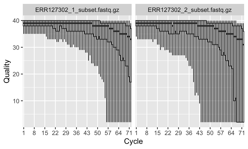
FIGURE 7.3: Per base sequence quality boxplot.
In our case, the x-axis in the plot is labeled as “cycle”. This is because in each sequencing “cycle” a fluorescently labeled nucleotide is added to complement the template sequence, and the sequencing machine identifies which nucleotide is added. Therefore, cycles correspond to bases/nucleotides along the read, and the number of cycles is equivalent to the read length.
Long sequences can have degraded quality towards the ends of the reads. Looking at quality distribution over base positions can help us decide to do trimming towards the end of the reads or not. A good sample will have median quality scores per base above 28. If scores are below 20 towards the ends, you can think about trimming the reads.
7.2.2 Sequence content per base/cycle
Per-base sequence content shows nucleotide proportions for each position. In a random sequencing library there should be no nucleotide bias and the lines should be almost parallel with each other. The code below shows how to get this plot. The resulting plot is shown in Figure 7.4.
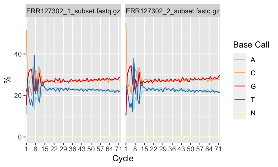
FIGURE 7.4: Percentage of nucleotide bases per position across different FASTQ files.
However, some types of sequencing libraries can produce a biased sequence composition. For example, in RNA-Seq, it is common to have bias at the beginning of the reads. This happens because of random primers annealing to the start of reads during RNA-Seq library preparation. These primers are not truly random, which leads to a variation at the beginning of the reads. Although RNA-seq experiments will usually have these biases, this will not affect the ability of measuring gene expression.
In addition, some libraries are inherently biased in their sequence composition. For example, in bisulfite sequencing experiments, most of the cytosines will be converted to thymines. This will create a difference in C and T base compositions over the read, however this type of difference is normal for bisulfite sequencing experiments.
7.2.3 Read frequency plot
This plot shows the degree of duplication for every read in the library. We show how to get this plot in the code snippet below and the resulting plot is in Figure 7.5. A high level of duplication, non-unique reads, is likely to indicate an enrichment bias. Technical duplicates arising from PCR artifacts could cause this. PCR is a common step in library preparation which creates many copies of the sequence fragment. In RNA-seq data, the non-unique read proportion can reach more than 20%. However, these duplications may stem from genes simply being expressed at high levels. This means that there will be many copies of transcripts and many copies of the same fragment. Since we cannot be sure these duplicated reads are due to PCR bias or an effect of high transcription, we should not remove duplicated reads in RNA-seq analysis. However, in ChIP-seq experiments duplicated reads are more likely to be due to PCR bias.
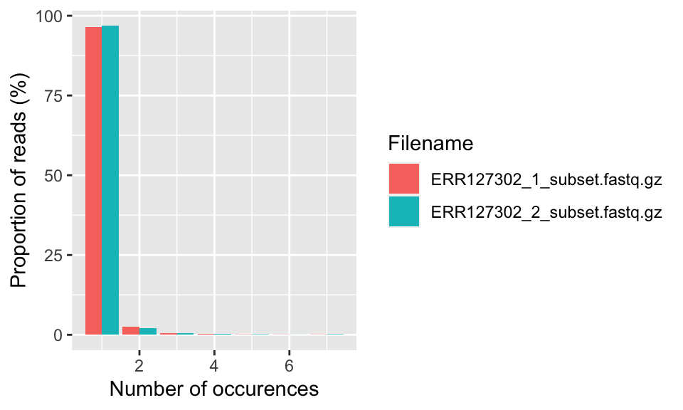
FIGURE 7.5: The percent of different duplication levels in FASTQ files. Most of the reads in all libraries have only one copy in this case.
7.2.4 Other quality metrics and QC tools
Over-represented k-mers along the reads can be an additional check. If there are such sequences it may point to adapter contamination and should be trimmed. Adapters are known sequences that are added to the ends of the reads. This kind of contamination could also be visible at “sequence content per base” plots. In addition, if you know the adapter sequences, you can match it to the end of the reads and trim them. The most popular tool for sequencing quality control is the fastQC tool (Andrews 2010), which is written in Java. It produces the plots that we described above in addition to k-mer overrepresentation and adapter overrepresentation plots. The R package fastqcr can run this Java tool and produce R-based plots and reports. This package simply calls the Java tool and parses its results. Below, we show how to do that.
library(fastqcr)

# install the FASTQC java tool
fastqc_install()

# call FASTQC and record the resulting statistics
# in fastqc_results folder
fastqc(fq.dir = folder,qc.dir = "fastqc_results")
Now that we have run FastQC on our fastq files, we can read the results to R and construct plots or reports. The gc_report() function can create an Rmarkdown-based report from FastQC output.
# view the report rendered by R functions
qc_report(qc.path="fastqc_results",
          result.file="reportFile", preview = TRUE)
Alternatively, we can read the results with qc_read() and make specific plots we are interested in with qc_plot().
# read QC results to R for one fastq file
qc <- qc_read("fastqc_results/ERR127302_1_subset_fastqc.zip")

# make plots, example "Per base sequence quality plot"
qc_plot(qc, "Per base sequence quality")
Apart from this, the bioconductor packages Rqc (de Souza, Carvalho, and Lopes-Cendes 2018) (see Rqc::rqcReport function), QuasR (Gaidatzis, Lerch, Hahne, et al. 2015) (see QuasR::qQCReport function), systemPipeR (Backman and Girke 2016) (see systemPipeR::seeFastq function), and ShortRead (Morgan, Anders, Lawrence, et al. 2009) (see ShortRead::report function) can all generate quality reports in a similar fashion to FastQC with some differences in plot content and number.
References
Backman, and Girke. 2016. “systemPipeR: NGS Workflow and Report Generation Environment.” BMC Bioinformatics 17 (1). https://doi.org/10.1186/s12859-016-1241-0.
de Souza, Carvalho, and Lopes-Cendes. 2018. “Rqc: A Bioconductor Package for Quality Control of High-Throughput Sequencing Data.” Journal of Statistical Software, Code Snippets 87 (2): 1–14. https://doi.org/10.18637/jss.v087.c02.
Gaidatzis, Lerch, Hahne, and Stadler. 2015. “QuasR: Quantification and Annotation of Short Reads in R.” Bioinformatics 31 (7): 1130–2. https://doi.org/10.1093/bioinformatics/btu781.
Morgan, Anders, Lawrence, Aboyoun, Pagès, and Gentleman. 2009. “ShortRead: A Bioconductor Package for Input, Quality Assessment and Exploration of High-Throughput Sequence Data.” Bioinformatics 25 (19): 2607–8. https://doi.org/10.1093/bioinformatics/btp450.