2.4 Data structures

R has multiple data structures. If you are familiar with Excel, you can think of a single Excel sheet as a table and data structures as building blocks of that table. Most of the time you will deal with tabular data sets or you will want to transform your raw data to a tabular data set, and you will try to manipulate this tabular data set in some way. For example, you may want to take sub-sections of the table or extract all the values in a column. For these and similar purposes, it is essential to know the common data structures in R and how they can be used. R deals with named data structures, which means you can give names to data structures and manipulate or operate on them using those names. It will be clear soon what we mean by this if “named data structures” does not ring a bell.

2.4.1 Vectors

Vectors are one of the core R data structures. It is basically a list of elements of the same type (numeric, character or logical). Later you will see that every column of a table will be represented as a vector. R handles vectors easily and intuitively. You can create vectors with the c() function, however that is not the only way. The operations on vectors will propagate to all the elements of the vectors.

x<-c(1,3,2,10,5)    #create a vector named x with 5 components
x = c(1,3,2,10,5)  
x

## [1]  1  3  2 10  5

y<-1:5              #create a vector of consecutive integers y
y+2                 #scalar addition

## [1] 3 4 5 6 7

2*y                 #scalar multiplication

## [1]  2  4  6  8 10

y^2                 #raise each component to the second power

## [1]  1  4  9 16 25

2^y                 #raise 2 to the first through fifth power

## [1]  2  4  8 16 32

y                   #y itself has not been unchanged

## [1] 1 2 3 4 5

y<-y*2
y                   #it is now changed

## [1]  2  4  6  8 10

r1<-rep(1,3)        # create a vector of 1s, length 3
length(r1)           #length of the vector

## [1] 3

class(r1)            # class of the vector

## [1] "numeric"

a<-1                # this is actually a vector length one

The standard assignment operator in R is <-. This operator is preferentially used in books and documentation. However, it is also possible to use the = operator for the assignment. We have an example in the above code snippet and throughout the book we use <- and = interchangeably for assignment.

2.4.2 Matrices

A matrix refers to a numeric array of rows and columns. You can think of it as a stacked version of vectors where each row or column is a vector. One of the easiest ways to create a matrix is to combine vectors of equal length using cbind(), meaning ‘column bind’.

x<-c(1,2,3,4)
y<-c(4,5,6,7)
m1<-cbind(x,y);m1

##      x y
## [1,] 1 4
## [2,] 2 5
## [3,] 3 6
## [4,] 4 7

t(m1)                # transpose of m1

##   [,1] [,2] [,3] [,4]
## x    1    2    3    4
## y    4    5    6    7

dim(m1)              # 2 by 5 matrix

## [1] 4 2

You can also directly list the elements and specify the matrix:

m2<-matrix(c(1,3,2,5,-1,2,2,3,9),nrow=3)
m2

##      [,1] [,2] [,3]
## [1,]    1    5    2
## [2,]    3   -1    3
## [3,]    2    2    9

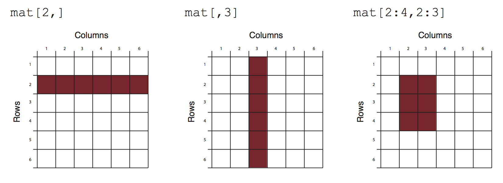
Matrices and the next data structure, data frames, are tabular data structures. You can subset them using [] and providing desired rows and columns to subset. Figure 2.1 shows how that works conceptually.

FIGURE 2.1: Slicing/subsetting of a matrix and a data frame.

2.4.3 Data frames

A data frame is more general than a matrix, in that different columns can have different modes (numeric, character, factor, etc.). A data frame can be constructed by the data.frame() function. For example, we illustrate how to construct a data frame from genomic intervals or coordinates.

chr <- c("chr1", "chr1", "chr2", "chr2")
strand <- c("-","-","+","+")
start<- c(200,4000,100,400)
end<-c(250,410,200,450)
mydata <- data.frame(chr,start,end,strand)
#change column names
names(mydata) <- c("chr","start","end","strand")
mydata # OR this will work too

##    chr start end strand
## 1 chr1   200 250      -
## 2 chr1  4000 410      -
## 3 chr2   100 200      +
## 4 chr2   400 450      +

mydata <- data.frame(chr=chr,start=start,end=end,strand=strand)
mydata

##    chr start end strand
## 1 chr1   200 250      -
## 2 chr1  4000 410      -
## 3 chr2   100 200      +
## 4 chr2   400 450      +

There are a variety of ways to extract the elements of a data frame. You can extract certain columns using column numbers or names, or you can extract certain rows by using row numbers. You can also extract data using logical arguments, such as extracting all rows that have a value in a column larger than your threshold.

mydata[,2:4] # columns 2,3,4 of data frame

##   start end strand
## 1   200 250      -
## 2  4000 410      -
## 3   100 200      +
## 4   400 450      +

mydata[,c("chr","start")] # columns chr and start from data frame

##    chr start
## 1 chr1   200
## 2 chr1  4000
## 3 chr2   100
## 4 chr2   400

mydata$start # variable start in the data frame

## [1]  200 4000  100  400

mydata[c(1,3),] # get 1st and 3rd rows

##    chr start end strand
## 1 chr1   200 250      -
## 3 chr2   100 200      +

mydata[mydata$start>400,] # get all rows where start>400

##    chr start end strand
## 2 chr1  4000 410      -

2.4.4 Lists

A list in R is an ordered collection of objects (components). A list allows you to gather a variety of (possibly unrelated) objects under one name. You can create a list with the list() function. Each object or element in the list has a numbered position and can have names. Below we show a few examples of how to create lists.

# example of a list with 4 components
# a string, a numeric vector, a matrix, and a scalar
w <- list(name="Fred",
       mynumbers=c(1,2,3),
       mymatrix=matrix(1:4,ncol=2),
       age=5.3)
w

## $name
## [1] "Fred"
## 
## $mynumbers
## [1] 1 2 3
## 
## $mymatrix
##      [,1] [,2]
## [1,]    1    3
## [2,]    2    4
## 
## $age
## [1] 5.3

You can extract elements of a list using the [[]], the double square-bracket, convention using either its position in the list or its name.

w[[3]] # 3rd component of the list

##      [,1] [,2]
## [1,]    1    3
## [2,]    2    4

w[["mynumbers"]] # component named mynumbers in list

## [1] 1 2 3

w$age

## [1] 5.3

2.4.5 Factors

Factors are used to store categorical data. They are important for statistical modeling since categorical variables are treated differently in statistical models than continuous variables. This ensures categorical data treated accordingly in statistical models.

features=c("promoter","exon","intron")
f.feat=factor(features)

An important thing to note is that when you are reading a data frame with read.table() or creating a data frame with data.frame() function, the character columns are stored as factors by default, to change this behavior you need to set stringsAsFactors=FALSE in read.table() and/or data.frame() function arguments.