6.4 Genomic intervals with more information: SummarizedExperiment class
As we have seen, genomic intervals can be mainly contained in a GRanges object.
It can also contain additional columns associated with each interval. Here
you can save information such as read counts or other scores associated with the
interval. However,
genomic data often have many layers. With GRanges you can have a table
associated with the intervals, but what happens if you have many tables and each
table has some metadata associated with it. In addition, rows and columns might
have additional annotation that cannot be contained by row or column names.
For these cases, the SummarizedExperiment class is ideal. It can hold multi-layered
tabular data associated with each genomic interval and the meta-data associated with
rows and columns, or associated with each table. For example, genomic intervals
associated with the SummarizedExperiment object can be gene locations, and
each tabular data structure can be RNA-seq read counts in a time course experiment.
Each table could represent different conditions in which experiments are performed.
The SummarizedExperiment class is outlined in the figure below (Figure 6.5 ).
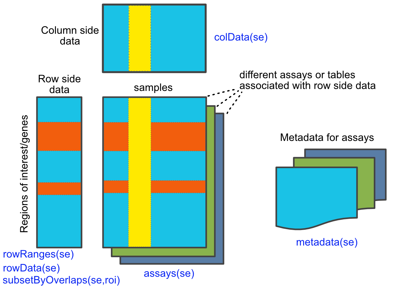
FIGURE 6.5: Overview of SummarizedExperiment class and functions. Adapted from the SummarizedExperiment package vignette.
6.4.1 Create a SummarizedExperiment object
Here we show how to create a basic SummarizedExperiment object. We will first
create a matrix of read counts. This matrix will represent read counts from
a series of RNA-seq experiments from different time points. Following that,
we create a GRanges object to represent the locations of the genes, and a table
for column annotations. This will include the names for the columns and any
other value we want to represent. Finally, we will create a SummarizedExperiment
object by combining all those pieces.
# simulate an RNA-seq read counts table
nrows <- 200
ncols <- 6
counts <- matrix(runif(nrows * ncols, 1, 1e4), nrows)

# create gene locations
rowRanges <- GRanges(rep(c("chr1", "chr2"), c(50, 150)),
                     IRanges(floor(runif(200, 1e5, 1e6)), width=100),
                     strand=sample(c("+", "-"), 200, TRUE),
                     feature_id=paste0("gene", 1:200))

# create table for the columns
colData <- DataFrame(timepoint=1:6,
                     row.names=LETTERS[1:6])


# create SummarizedExperiment object
se=SummarizedExperiment(assays=list(counts=counts),
                     rowRanges=rowRanges, colData=colData)

se
## class: RangedSummarizedExperiment
## dim: 200 6
## metadata(0):
## assays(1): counts
## rownames: NULL
## rowData names(1): feature_id
## colnames(6): A B ... E F
## colData names(1): timepoint6.4.2 Subset and manipulate the SummarizedExperiment object
Now that we have a SummarizedExperiment object, we can subset it and extract/change
parts of it.
6.4.2.1 Extracting parts of the object
colData() and rowData() extract the column-associated and row-associated
tables. metaData() extracts the meta-data table if there is any table associated.
## DataFrame with 6 rows and 1 column
##   timepoint
##   <integer>
## A         1
## B         2
## C         3
## D         4
## E         5
## F 6## DataFrame with 200 rows and 1 column
## feature_id
## <character>
## 1 gene1
## 2 gene2
## 3 gene3
## 4 gene4
## 5 gene5
## ... ...
## 196 gene196
## 197 gene197
## 198 gene198
## 199 gene199
## 200 gene200To extract the main table or tables that contain the values of interest such
as read counts, we must use the assays() function. This returns a list of
DataFrame objects associated with the object.
## List of length 1
## names(1): counts
You can use names with $ or [] notation to extract specific tables from the list.
6.4.2.2 Subsetting
Subsetting is easy using [ ] notation. This is similar to the way we
subset data frames or matrices.
## class: RangedSummarizedExperiment
## dim: 5 3
## metadata(0):
## assays(1): counts
## rownames: NULL
## rowData names(1): feature_id
## colnames(3): A B C
## colData names(1): timepoint
One can also use the $ operator to subset based on colData() columns. You can
extract certain samples or in our case, time points.
In addition, as SummarizedExperiment objects are GRanges objects on steroids,
they support all of the findOverlaps() methods and associated functions that
work on GRanges objects.
# Subset for only rows which are in chr1:100,000-1,100,000
roi <- GRanges(seqnames="chr1", ranges=100000:1100000)
subsetByOverlaps(se, roi)
## class: RangedSummarizedExperiment
## dim: 50 6
## metadata(0):
## assays(1): counts
## rownames: NULL
## rowData names(1): feature_id
## colnames(6): A B ... E F
## colData names(1): timepoint