5.7 Assessing the performance of our model

We have to define some metrics to see if our model worked. The algorithm is trying to reduce the classification error, or in other words it is trying to increase the training accuracy. For the assessment of performance, there are other different metrics to consider. All the metrics for 2-class classification depend on the table below, which shows the number of true positives (TP), false positives (FP), true negatives (TN) and false negatives (FN), similar to a table we used in the hypothesis testing section in the statistics chapter previously.

	Actual CIMP	Actual noCIMP
Predicted as CIMP	True Positives (TP)	False Positive (FP)
Predicted as noCIMP	False Positives (FN)	True negatives (TN)

Accuracy is the first metric to look at. This metric is simply \((TP+TN)/(TP+TN+FP+FN)\) and shows the proportion of times we were right. There are other accuracy metrics that are important and output by caret functions. We will go over some of them here.

Precision, \(TP/(TP+FP)\), is about the confidence we have on our CIMP calls. If our method is very precise, we will have low false positives. That means every time we call a CIMP event, we would be relatively certain it is not a false positive.

Sensitivity, \(TP/(TP+FN)\), is how often we miss CIMP cases and call them as noCIMP. Making fewer mistakes in noCIMP cases will increase our sensitivity. You can think of sensitivity also in a sick/healthy context. A highly sensitive method will be good at classifying sick people when they are indeed sick.

Specificity, \(TN/(TN+FP)\), is about how sure we are when we call something noCIMP. If our method is not very specific, we would call many patients CIMP, while in fact, they did not have the subtype. In the sick/healthy context, a highly specific method will be good at not calling healthy people sick.

An alternative to accuracy we showed earlier is “balanced accuracy”. Accuracy does not perform well when classes have very different numbers of samples (class imbalance). For example, if you have 90 CIMP cases and 10 noCIMP cases, classifying all the samples as CIMP gives 0.9 accuracy score by default. Using the “balanced accuracy” metric can help in such situations. This is simply \((Precision+Sensitivity)/2\). In this case above with the class imbalance scenario, the “balanced accuracy” would be 0.5. Another metric that takes into account accuracy that could be generated by chance is the “Kappa statistic” or “Cohen’s Kappa”. This metric includes expected accuracy, which is affected by class imbalance in the training set and provides a metric corrected by that.

In the k-NN example above, we trained and tested on the same data. The model returned the predicted labels for our training. We can calculate the accuracy metrics using the caret::confusionMatrix() function. This is sometimes called training accuracy. If you take \(1-accuracy\), it will be the “training error”.

# get k-NN prediction on the training data itself, with k=5
knnFit=knn3(x=training[,-1], # training set
            y=training[,1], # training set class labels
            k=5)

# predictions on the training set
trainPred=predict(knnFit,training[,-1],type="class")

# compare the predicted labels to real labels
# get different performance metrics
confusionMatrix(data=training[,1],reference=trainPred)

## Confusion Matrix and Statistics
## 
##           Reference
## Prediction CIMP noCIMP
##     CIMP     65      0
##     noCIMP    2     63
##                                           
##                Accuracy : 0.9846          
##                  95% CI : (0.9455, 0.9981)
##     No Information Rate : 0.5154          
##     P-Value [Acc > NIR] : <2e-16          
##                                           
##                   Kappa : 0.9692          
##                                           
##  Mcnemar's Test P-Value : 0.4795          
##                                           
##             Sensitivity : 0.9701          
##             Specificity : 1.0000          
##          Pos Pred Value : 1.0000          
##          Neg Pred Value : 0.9692          
##              Prevalence : 0.5154          
##          Detection Rate : 0.5000          
##    Detection Prevalence : 0.5000          
##       Balanced Accuracy : 0.9851          
##                                           
##        'Positive' Class : CIMP            
## 

Now, let us see what our test set accuracy looks like again using the knn function and the confusionMatrix() function on the predicted and real classes.

# predictions on the test set, return class labels
testPred=predict(knnFit,testing[,-1],type="class")

# compare the predicted labels to real labels
# get different performance metrics
confusionMatrix(data=testing[,1],reference=testPred)

## Confusion Matrix and Statistics
## 
##           Reference
## Prediction CIMP noCIMP
##     CIMP     27      0
##     noCIMP    2     25
##                                           
##                Accuracy : 0.963           
##                  95% CI : (0.8725, 0.9955)
##     No Information Rate : 0.537           
##     P-Value [Acc > NIR] : 2.924e-12       
##                                           
##                   Kappa : 0.9259          
##                                           
##  Mcnemar's Test P-Value : 0.4795          
##                                           
##             Sensitivity : 0.9310          
##             Specificity : 1.0000          
##          Pos Pred Value : 1.0000          
##          Neg Pred Value : 0.9259          
##              Prevalence : 0.5370          
##          Detection Rate : 0.5000          
##    Detection Prevalence : 0.5000          
##       Balanced Accuracy : 0.9655          
##                                           
##        'Positive' Class : CIMP            
## 

Test set accuracy is not as good as the training accuracy, which is usually the case. That is why the best way to evaluate performance is to use test data that is not used by the model for training. That gives you an idea about real-world performance where the model will be used to predict data that is not previously seen.

5.7.1 Receiver Operating Characteristic (ROC) curves

One important and popular metric when evaluating performance is looking at receiver operating characteristic (ROC) curves. The ROC curve is created by evaluating the class probabilities for the model across a continuum of thresholds. Typically, in the case of two-class classification, the methods return a probability for one of the classes. If that probability is higher than \(0.5\), you call the label, for example, class A. If less than \(0.5\), we call the label class B. However, we can move that threshold and change what we call class A or B. For each candidate threshold, the resulting sensitivity and 1-specificity are plotted against each other. The best possible prediction would result in a point in the upper left corner, representing 100% sensitivity (no false negatives) and 100% specificity (no false positives). For the best model, the curve will be almost like a square. Since this is important information, area under the curve (AUC) is calculated. This is a quantity between 0 and 1, and the closer to 1, the better the performance of your classifier in terms of sensitivity and specificity. For an uninformative classification model, AUC will be \(0.5\). Although, ROC curves are initially designed for two-class problems, later extensions made it possible to use ROC curves for multi-class problems.

ROC curves can also be used to determine alternate cutoffs for class probabilities for two-class problems. However, this will always result in a trade-off between sensitivity and specificity. Sometimes it might be desirable to limit the number of false positives because making such mistakes would be too costly for the individual cases. For example, if predicted with a certain disease, you might be recommended to have surgery. However, if your classifier has a relatively high false positive rate, low specificity, you might have surgery for no reason. Typically, you want your classification model to have high specificity and sensitivity, which may not always be possible in the real world. You might have to choose what is more important for a specific problem and try to increase that.

Next, we will show how to use ROC curves for our k-NN application. The method requires classification probabilities in the format where 0 probability denotes class “noCIMP” and probability 1 denotes class “CIMP”. This way the ROC curve can be drawn by varying the probability cutoff for calling class a “noCIMP” or “CIMP”. Below we are getting a similar probability from k-NN, but we have to transform it to the format we described above. Then, we feed those class probabilities to the pROC::roc() function to calculate the ROC curve and the area-under-the-curve. The resulting ROC curve is shown in Figure 5.3.

library(pROC)

# get k-NN class probabilities
# prediction probabilities on the test set
testProbs=predict(knnFit,testing[,-1])

# get the roc curve
rocCurve <- pROC::roc(response = testing[,1],
                predictor = testProbs[,1],
              ## This function assumes that the second
              ## class is the class of interest, so we
              ## reverse the labels.
              levels = rev(levels(testing[,1])))
# plot the curve
plot(rocCurve, legacy.axes = TRUE)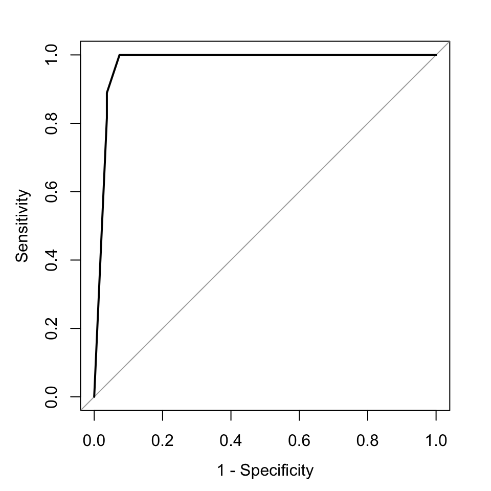

FIGURE 5.3: ROC curve for k-NN.

# return area under the curve
pROC::auc(rocCurve)

## Area under the curve: 0.976