11.1 Use case: Multi-omics data from colorectal cancer
The examples in this chapter will use the following data: a set of 121 tumors from the TCGA (Weinstein, Collisson, Mills, et al. 2013) colorectal cancer cohort. The tumors have been profiled for gene expression using RNA-seq, mutations using Exome-seq, and copy number variations using genotyping arrays. Projects such as TCGA have turbocharged efforts to sub-divide cancer into subtypes. Although two tumors arise in the colon, they may have distinct molecular profiles, which is important for treatment decisions. The subset of tumors used in this chapter belong to two distinct molecular subtypes defined by the Colorectal Cancer Subtyping Consortium (Guinney, Dienstmann, Wang, et al. 2015), CMS1 and CMS3. The following code snippets load this multi-omics data from the companion package, starting with gene expression data from RNA-seq (see Chapter 8). Below we are reading the RNA-seq data from the compGenomRData package.
# read in the csv from the companion package as a data frame
csvfile <- system.file("extdata", "multi-omics", "COREAD_CMS13_gex.csv",
                       package="compGenomRData")
x1 <- read.csv(csvfile, row.names=1)
# Fix the gene names in the data frame
rownames(x1) <- sapply(strsplit(rownames(x1), "\\|"), function(x) x[1])
# Output a table
knitr::kable(head(t(head(x1))), caption="Example gene expression data (head)")| RNF113A | S100A13 | AP3D1 | ATP6V1G1 | UBQLN4 | TPPP3 | |
|---|---|---|---|---|---|---|
| TCGA.A6.2672 | 21.19567 | 19.72600 | 11.53022 | 0.00000 | 15.35637 | 12.76747 |
| TCGA.A6.3809 | 21.50866 | 18.65729 | 12.98830 | 14.12675 | 19.62208 | 0.00000 |
| TCGA.A6.5661 | 20.08072 | 18.97034 | 10.83759 | 15.31325 | 0.00000 | 0.00000 |
| TCGA.A6.5665 | 0.00000 | 11.88336 | 10.24248 | 19.79300 | 0.00000 | 0.00000 |
| TCGA.A6.6653 | 0.00000 | 12.07753 | 0.00000 | 0.00000 | 0.00000 | 0.00000 |
| TCGA.A6.6780 | 0.00000 | 12.99128 | 0.00000 | 19.96976 | 13.17618 | 11.58742 |
| Table @ref(tab | :moloadMult | iomicsGE) s | hows the he | ad of the g | ene express | ion matrix. The rows correspond to patients, referred to by their TCGA identifier, as the first column of the table. Columns represent the genes, and the values are RPKM expression values. The column names are the names or symbols of the genes. |
| The details abo | ut how thes | e expressio | n values ar | e calculate | d are in Ch | apter 8. |
We first read mutation data with the following code snippet.
# read in the csv from the companion package as a data frame
csvfile <- system.file("extdata", "multi-omics", "COREAD_CMS13_muts.csv",
                       package="compGenomRData")
x2 <- read.csv(csvfile, row.names=1)
# Set mutation data to be binary (so if a gene has more than 1 mutation,
# we only count one)
x2[x2>0]=1
# output a table
knitr::kable(head(t(head(x2))), caption="Example mutation data (head)")| TTN | TP53 | APC | KRAS | SYNE1 | MUC16 | |
|---|---|---|---|---|---|---|
| TCGA.A6.2672 | 1 | 0 | 0 | 0 | 1 | 1 |
| TCGA.A6.3809 | 1 | 0 | 0 | 0 | 0 | 0 |
| TCGA.A6.5661 | 1 | 0 | 0 | 0 | 1 | 1 |
| TCGA.A6.5665 | 1 | 0 | 0 | 0 | 1 | 1 |
| TCGA.A6.6653 | 1 | 0 | 0 | 1 | 0 | 0 |
| TCGA.A6.6780 | 1 | 0 | 0 | 0 | 0 | 1 |
| Table @ref(tab | :moloa | dMultio | micsMU | T) show | s the mu | tations of these tumors (mutations were introduced in Chapter 1). In the mutation matrix, each cell is a binary 1/0, indicating whether or not a tumor has a non-synonymous mutation in the gene indicated by the column. These types of mutations change the aminoacid sequence, therefore they are likely to change the function of the protein. |
Next, we read copy number data with the following code snippet.
# read in the csv from the companion package as a data frame
csvfile <- system.file("extdata", "multi-omics", "COREAD_CMS13_cnv.csv",
                       package="compGenomRData")
x3 <- read.csv(csvfile, row.names=1)
# output a table
knitr::kable(head(t(head(x3))),
caption="Example copy number data for CRC samples")| 8p23.2 | 8p23.3 | 8p23.1 | 8p21.3 | 8p12 | 8p22 | |
|---|---|---|---|---|---|---|
| TCGA.A6.2672 | 0 | 0 | 0 | 0 | 0 | 0 |
| TCGA.A6.3809 | 0 | 0 | 0 | 0 | 0 | 0 |
| TCGA.A6.5661 | 0 | 0 | 0 | 0 | 0 | 0 |
| TCGA.A6.5665 | 0 | 0 | 0 | 0 | 0 | 0 |
| TCGA.A6.6653 | 0 | 0 | 0 | 0 | 0 | 0 |
| TCGA.A6.6780 | 0 | 0 | 0 | 0 | 0 | 0 |
| Finally, table | @ref(tab | :moloadMu | ltiomicsC | NV) shows | GISTIC | scores (Mermel, Schumacher, Hill, et al. 2011) for copy number alterations in these tumors. During transformation from healthy cells to cancer cells, the genome sometimes undergoes large-scale instability; large segments of the genome might be replicated or lost. This will be reflected in each segment’s “copy number”. In this matrix, each column corresponds to a chromosome segment, and the value of the cell is a real-valued score indicating if this segment has been amplified (copied more) or lost, relative to a non-cancer control from the same patient. |
Each of the data types (gene expression, mutations, copy number variation) on its own, provides some signal which allows us to somewhat separate the samples into the two different subtypes. In order to explore these relations, we must first obtain the subtypes of these tumors. The following code snippet reads these, also from the companion package:
# read in the csv from the companion package as a data frame
csvfile <- system.file("extdata", "multi-omics", "COREAD_CMS13_subtypes.csv",
                       package="compGenomRData")
covariates <- read.csv(csvfile, row.names=1)
# Fix the TCGA identifiers so they match up with the omics data
rownames(covariates) <- gsub(pattern = '-', replacement = '\\.',
                             rownames(covariates))
covariates <- covariates[colnames(x1),]
# create a dataframe which will be used to annotate later graphs
anno_col <- data.frame(cms=as.factor(covariates$cms_label))
rownames(anno_col) <- rownames(covariates)
Before proceeding with any multi-omics integration analysis which might obscure the underlying data, it is important to take a look at each omic data type on its own, and in this case in particular, to examine their relation to the underlying condition, i.e. the cancer subtype. A great way to get an eagle-eye view of such large data is using heatmaps (see Chapter 4 for more details).
We will first check the gene expression data in relation to the subtypes. One way of doing that is plotting a heatmap and clustering the tumors, while displaying a color annotation atop the heatmap, indicating which subtype each tumor belongs to. This is shown in Figure 11.1, which is generated by the following code snippet:
pheatmap::pheatmap(x1,
                   annotation_col = anno_col,
                   show_colnames = FALSE,
                   show_rownames = FALSE,
                   main="Gene expression data")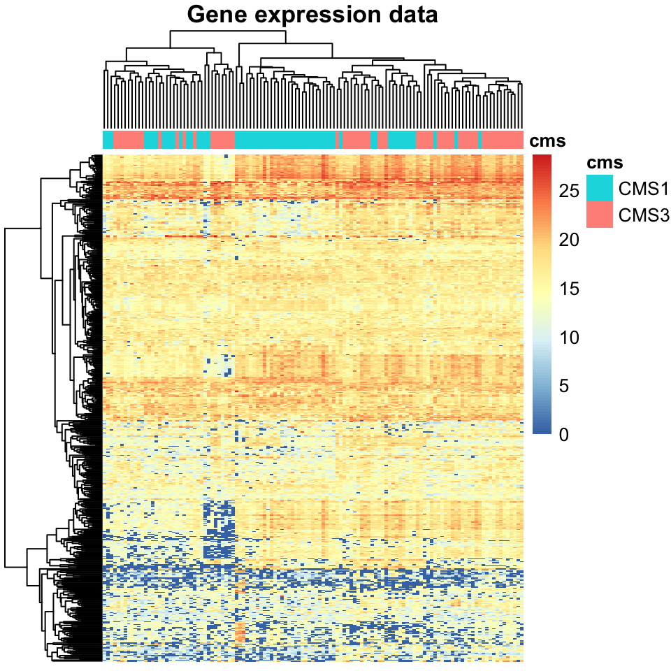
FIGURE 11.1: Heatmap of gene expression data for colorectal cancers.
In Figure 11.1, each column is a tumor, and each row is a gene. The values in the cells are FPKM values. There is another band above the heatmap annotating each column (tumor) with its corresponding subtype. The tumors are clustered using hierarchical clustering denoted by the dendrogram above the heatmap, according to which the columns (tumors) are ordered. While this ordering corresponds somewhat to the subtypes, it would not be possible to cut this dendrogram in a way which achieves perfect separation between the subtypes.
Next we repeat the same exercise using the mutation data. The following snippet generates Figure 11.2:
pheatmap::pheatmap(x2,
                   annotation_col = anno_col,
                   show_colnames = FALSE,
                   show_rownames = FALSE,
                   main="Mutation data")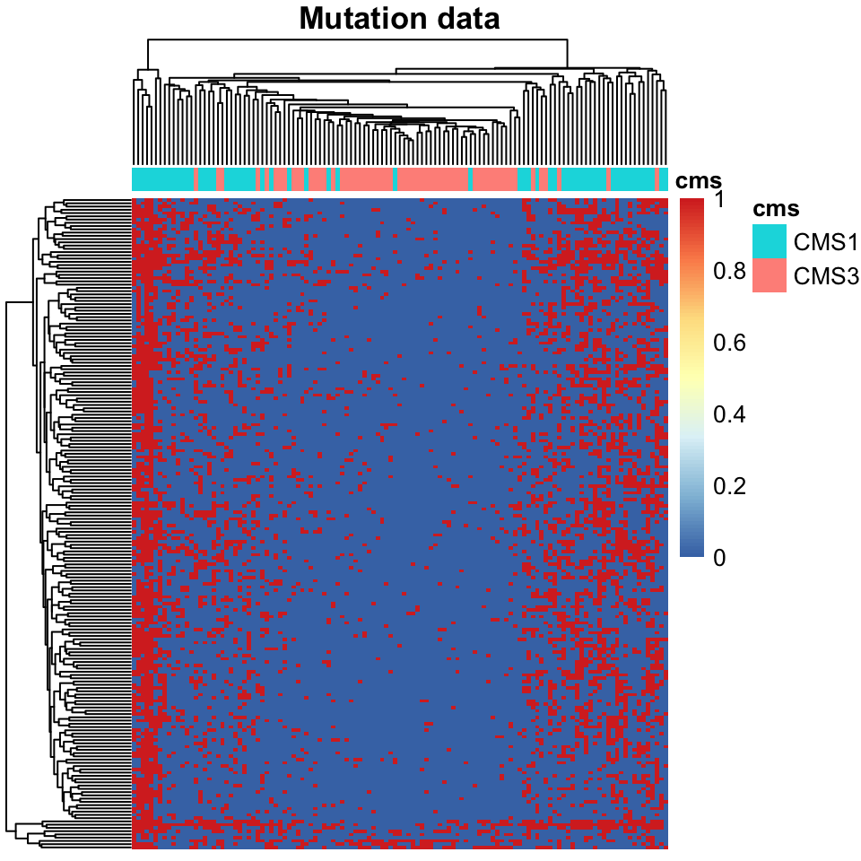
FIGURE 11.2: Heatmap of mutation data for colorectal cancers.
An examination of Figure 11.2 shows that tumors clustered and ordered by mutation data correspond very closely to their CMS subtypes. However, one should be careful in drawing conclusions about this result. Upon closer examination, you might notice that the separating factor seems to be that CMS1 tumors have significantly more mutations than do CMS3 tumors. This, rather than mutations in a specific genes, seems to be driving this clustering result. Nevertheless, this hyper-mutated status is an important indicator for this subtype.
Finally, we look into copy number variation data and try to see if clustered samples are in concordance with subtypes. The following code snippet generates Figure 11.3:
pheatmap::pheatmap(x3,
                   annotation_col = anno_col,
                   show_colnames = FALSE,
                   show_rownames = FALSE,
                   main="Copy number data")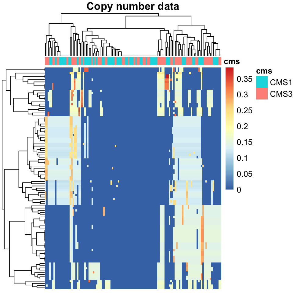
FIGURE 11.3: Heatmap of copy number variation data, colorectal cancers.
The interpretation of Figure 11.3 is left as an exercise for the reader.
It is clear that while there is some “signal” in each of these omics types, as is evident from these heatmaps, it is equally clear that none of these omics types completely and on its own explains the subtypes. Each omics type provides but a glimpse into what makes each of these tumors different from a healthy cell. Through the rest of this chapter, we will demonstrate how analyzing the gene expression, mutations, and copy number variations, in tandem, we will be able to get a better picture of what separates these cancer subtypes.
The next section will describe latent variable models for multi-omics integrations. Latent variable models are a form of dimensionality reduction (see Chapter 4). Each omics data type is “big data” in its own right; a typical RNA-seq experiment profiles upwards of 50 thousand different transcripts. The difficulties in handling large data matrices are only exacerbated by the introduction of more omics types into the analysis, as we are suggesting here. In order to overcome these challenges, latent variable models are a powerful way to reduce the dimensionality of the data down to a manageable size.
References
Guinney, Dienstmann, Wang, et al. 2015. “The consensus molecular subtypes of colorectal cancer.” Nat. Med. 21 (11): 1350–6.
Mermel, Schumacher, Hill, Meyerson, Beroukhim, and Getz. 2011. “GISTIC2. 0 Facilitates Sensitive and Confident Localization of the Targets of Focal Somatic Copy-Number Alteration in Human Cancers.” Genome Biology 12 (4): R41.
Weinstein, Collisson, Mills, et al. 2013. “The Cancer Genome Atlas Pan-Cancer analysis project.” Nat. Genet. 45 (10): 1113–20.