5.15 Predicting continuous variables: Regression with machine learning
Until now, we only considered methods that can help us predict class labels. However, all the methods we have shown can also be used to predict continuous variables. In this case, the methods will try to optimize the prediction in error which is usually in the form of the sum of squared errors (SSE): \(SSE=\sum (Y-f(X))^2\), where \(Y\) is the continuous response variable and \(f(X)\) is the outcome of the machine learning model.
In this section, we are going to show how to use a supervised learning method for regression. All the methods we have introduced previously in the context of classification can also do regression. Technically, this is just a simple change in the cost function format and the optimization step still tries to optimize the parameters of the cost function. In many cases, if your response variable is numeric, methods in the caret package will automatically apply regression.
5.15.1 Use case: Predicting age from DNA methylation
We will demonstrate random forest regression using a different data set which has a continuous response variable. This time we are going to try to predict the age of individuals from their DNA methylation levels. Methylation is a DNA modification which has implications in gene regulation and cell state. We have introduced DNA methylation in depth in Chapters 1 and 10, however for now, what we need to know is that there are about 24 million CpG dinucleotides in the human genome. Their methylation status can be measured with quantitative assays and the value is between 0 and 1. If it is 0, the CpG is not methylated in any of the cells in the sample, and if it is 1, the CpG is methylated in all the cells of the sample. It has been shown that methylation is predictive of the age of the individual that the sample is taken from (Numata, Ye, Hyde, et al. 2012; Horvath 2013). Now, we will try to test that with a data set containing hundreds of individuals, their age, and methylation values for ~27000 CpGs. We first read in the files and construct a training set.
5.15.2 Reading and processing the data
Let us first read in the data. When we run the summary and histogram we see that the methylation values are between \(0\) and \(1\) and there are \(108\) samples (see Figure 5.16 ). Typically, methylation values have bimodal distribution. In this case many of them have values around \(0\) and the second-most frequent value bracket is around \(0.9\).
# file path for CpG methylation and age
fileMethAge=system.file("extdata",
                      "CpGmeth2Age.rds",
                      package="compGenomRData")

# read methylation-age table
ameth=readRDS(fileMethAge)
dim(ameth)
## [1] 108 27579## Age cg26211698 cg03790787
## Min. :-0.4986 Min. :0.01223 Min. :0.05001
## 1st Qu.:-0.4027 1st Qu.:0.01885 1st Qu.:0.07818
## Median :18.8466 Median :0.02269 Median :0.08964
## Mean :25.9083 Mean :0.02483 Mean :0.09300
## 3rd Qu.:49.6110 3rd Qu.:0.02888 3rd Qu.:0.10423
## Max. :83.6411 Max. :0.04883 Max. :0.16271# plot histogram of methylation values
hist(unlist(ameth[,-1]),border="white",
col="cornflowerblue",main="",xlab="methylation values")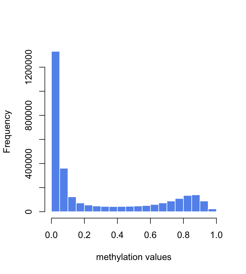
FIGURE 5.16: Histogram of methylation values in the training set for age prediction.
There are \(~27000\) predictor variables. We can remove the ones that have low variation across samples. In this case, the methylation values are between \(0\) and \(1\). The CpGs that have low variation are not likely to have any association with age; they could simply be technical variation of the experiment. We will remove CpGs that have less than 0.1 standard deviation.
## [1] 108 22905.15.3 Running random forest regression
Now we can use random forest regression to predict the age from methylation values. We are then going to plot the predicted vs. observed ages and see how good our predictions are. The resulting plots are shown in Figure 5.17.
set.seed(18)

par(mfrow=c(1,2))

# we are not going to do any cross-validatin
# and rely on OOB error
trctrl <- trainControl(method = "none")

# we will now train random forest model
rfregFit <- train(Age~.,
               data = ameth,
               method = "ranger",
               trControl=trctrl,
               # calculate importance
               importance="permutation",
               tuneGrid = data.frame(mtry=50,
                                     min.node.size = 5,
                                     splitrule="variance")
               )
# plot Observed vs OOB predicted values from the model
plot(ameth$Age,rfregFit$finalModel$predictions,
     pch=19,xlab="observed Age",
     ylab="OOB predicted Age")
mtext(paste("R-squared",
            format(rfregFit$finalModel$r.squared,digits=2)))

# plot residuals
plot(ameth$Age,(rfregFit$finalModel$predictions-ameth$Age),
     pch=18,ylab="residuals (predicted-observed)",
     xlab="observed Age",col="blue3")
abline(h=0,col="red4",lty=2)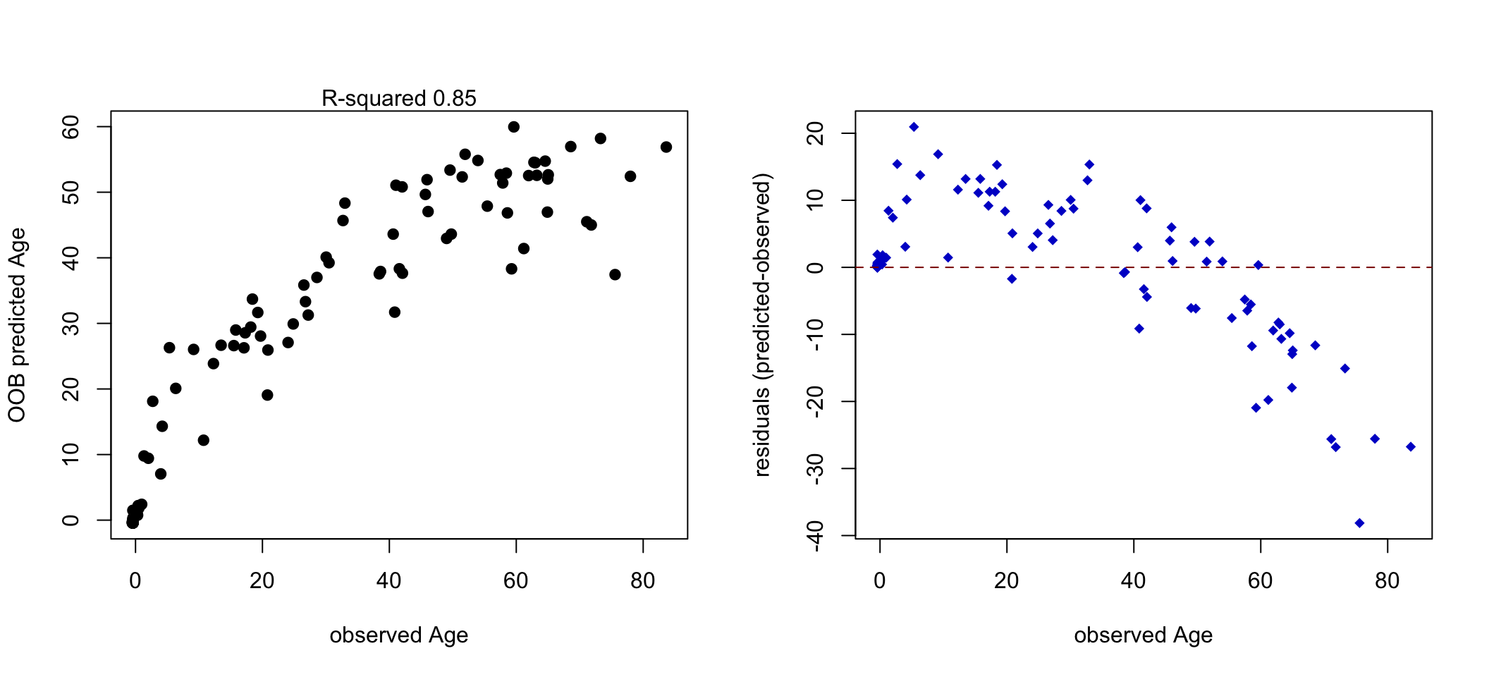
FIGURE 5.17: Observed vs. predicted age (Left). Residual plot showing that for older people the error increases (Right).
In this instance, we are using OOB errors and \(R^2\) value which shows how the model performs on OOB samples. The model can capture the general trend and it has acceptable OOB performance. It is not perfect as it makes errors on average close to 10 years when predicting the age, and the errors are more severe for older people (Figure 5.17). This could be due to having fewer older people to model or missing/inadequate predictor variables. However, everything we discussed in classification applies here. We had even fewer data points than the classification problem, so we did not do a split for a test data set. However, this should also be done for regression problems, especially when we are going to compare the performance of different models or want to have a better idea of the real-world performance of our model. We might also be interested in which variables are most important as in the classification problem; we can use the caret:varImp() function to get access to random-forest-specific variable importance metrics.
References
Horvath. 2013. “DNA Methylation Age of Human Tissues and Cell Types.” Genome Biology 14 (10): 3156.
Numata, Ye, Hyde, et al. 2012. “DNA Methylation Signatures in Development and Aging of the Human Prefrontal Cortex.” The American Journal of Human Genetics 90 (2): 260–72.