3.3 Relationship between variables: Linear models and correlation
In genomics, we would often need to measure or model the relationship between variables. We might want to know about expression of a particular gene in liver in relation to the dosage of a drug that patient receives. Or, we may want to know DNA methylation of a certain locus in the genome in relation to the age of the sample donor. Or, we might be interested in the relationship between histone modifications and gene expression. Is there a linear relationship, the more histone modification the more the gene is expressed ?
In these situations and many more, linear regression or linear models can be used to model the relationship with a “dependent” or “response” variable (expression or methylation in the above examples) and one or more “independent” or “explanatory” variables (age, drug dosage or histone modification in the above examples). Our simple linear model has the following components.
\[ Y= \beta_0+\beta_1X + \epsilon \]
In the equation above, \(Y\) is the response variable and \(X\) is the explanatory variable. \(\epsilon\) is the mean-zero error term. Since the line fit will not be able to precisely predict the \(Y\) values, there will be some error associated with each prediction when we compare it to the original \(Y\) values. This error is captured in the \(\epsilon\) term. We can alternatively write the model as follows to emphasize that the model approximates \(Y\), in this case notice that we removed the \(\epsilon\) term: \(Y \sim \beta_0+\beta_1X\).
The plot below in Figure 3.12 shows the relationship between histone modification (trimethylated forms of histone H3 at lysine 4, aka H3K4me3) and gene expression for 100 genes. The blue line is our model with estimated coefficients (\(\hat{y}=\hat{\beta}_0 + \hat{\beta}_1X\), where \(\hat{\beta}_0\) and \(\hat{\beta}_1\) are the estimated values of \(\beta_0\) and \(\beta_1\), and \(\hat{y}\) indicates the prediction). The red lines indicate the individual errors per data point, indicated as \(\epsilon\) in the formula above.
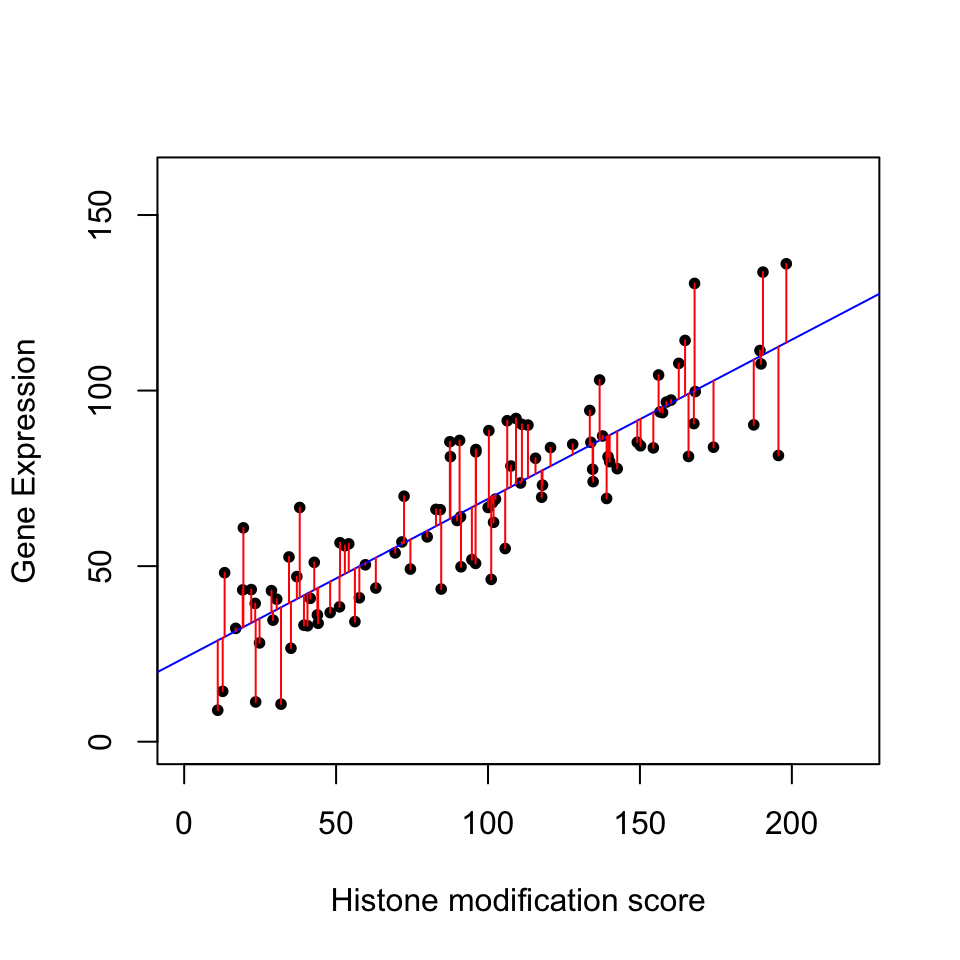
FIGURE 3.12: Relationship between histone modification score and gene expression. Increasing histone modification, H3K4me3, seems to be associated with increasing gene expression. Each dot is a gene
There could be more than one explanatory variable. We then simply add more \(X\) and \(\beta\) to our model. If there are two explanatory variables our model will look like this:
\[ Y= \beta_0+\beta_1X_1 +\beta_2X_2 + \epsilon \]
In this case, we will be fitting a plane rather than a line. However, the fitting process which we will describe in the later sections will not change for our gene expression problem. We can introduce one more histone modification, H3K27me3. We will then have a linear model with 2 explanatory variables and the fitted plane will look like the one in Figure 3.13. The gene expression values are shown as dots below and above the fitted plane. Linear regression and its extensions which make use of other distributions (generalized linear models) are central in computational genomics for statistical tests. We will see more of how regression is used in statistical hypothesis testing for computational genomics in Chapters 8 and 10.
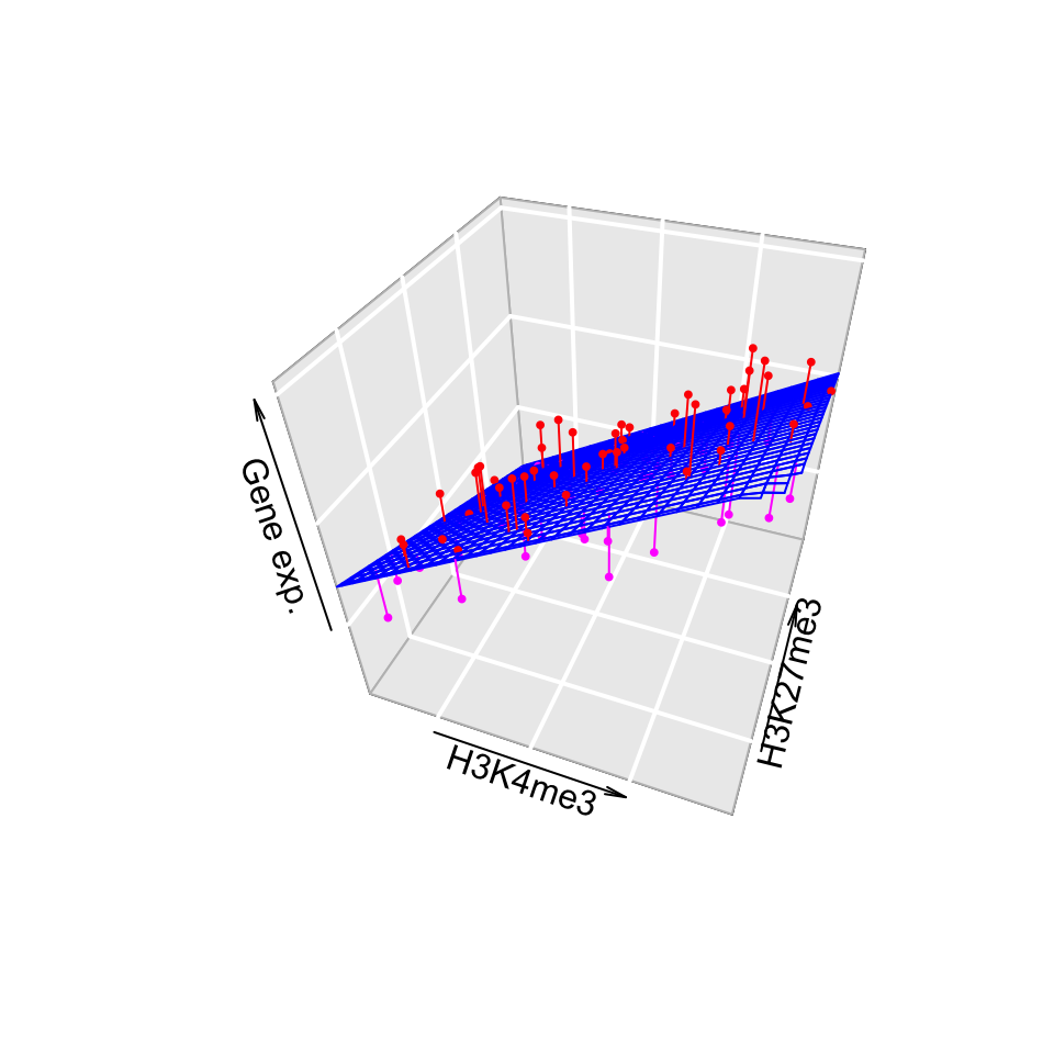
FIGURE 3.13: Association of gene expression with H3K4me3 and H3K27me3 histone modifications.
3.3.0.1 Matrix notation for linear models
We can naturally have more explanatory variables than just two. The formula below has \(n\) explanatory variables.
\[Y= \beta_0+\beta_1X_1+\beta_2X_2 + \beta_3X_3 + .. + \beta_nX_n +\epsilon\]
If there are many variables, it would be easier to write the model in matrix notation. The matrix form of linear model with two explanatory variables will look like the one below. The first matrix would be our data matrix. This contains our explanatory variables and a column of 1s. The second term is a column vector of \(\beta\) values. We also add a vector of error terms, \(\epsilon\)s, to the matrix multiplication.
\[ \mathbf{Y} = \left[\begin{array}{rrr} 1 & X_{1,1} & X_{1,2} \\ 1 & X_{2,1} & X_{2,2} \\ 1 & X_{3,1} & X_{3,2} \\ 1 & X_{4,1} & X_{4,2} \end{array}\right] % \left[\begin{array}{rrr} \beta_0 \\ \beta_1 \\ \beta_2 \end{array}\right] % + \left[\begin{array}{rrr} \epsilon_1 \\ \epsilon_2 \\ \epsilon_3 \\ \epsilon_0 \end{array}\right] \]
The multiplication of the data matrix and \(\beta\) vector and addition of the error terms simply results in the following set of equations per data point:
\[ \begin{aligned} Y_1= \beta_0+\beta_1X_{1,1}+\beta_2X_{1,2} +\epsilon_1 \\ Y_2= \beta_0+\beta_1X_{2,1}+\beta_2X_{2,2} +\epsilon_2 \\ Y_3= \beta_0+\beta_1X_{3,1}+\beta_2X_{3,2} +\epsilon_3 \\ Y_4= \beta_0+\beta_1X_{4,1}+\beta_2X_{4,2} +\epsilon_4 \end{aligned} \]
This expression involving the multiplication of the data matrix, the \(\beta\) vector and vector of error terms (\(\epsilon\)) could be simply written as follows.
\[Y=X\beta + \epsilon\]
In the equation, above \(Y\) is the vector of response variables, \(X\) is the data matrix, and \(\beta\) is the vector of coefficients. This notation is more concise and often used in scientific papers. However, this also means you need some understanding of linear algebra to follow the math laid out in such resources.
3.3.1 How to fit a line
At this point a major question is left unanswered: How did we fit this line? We basically need to define \(\beta\) values in a structured way. There are multiple ways of understanding how to do this, all of which converge to the same end point. We will describe them one by one.
3.3.1.1 The cost or loss function approach
This is the first approach and in my opinion is easiest to understand. We try to optimize a function, often called the “cost function” or “loss function”. The cost function is the sum of squared differences between the predicted \(\hat{Y}\) values from our model and the original \(Y\) values. The optimization procedure tries to find \(\beta\) values that minimize this difference between the reality and predicted values.
\[min \sum{(y_i-(\beta_0+\beta_1x_i))^2}\]
Note that this is related to the error term, \(\epsilon\), we already mentioned above. We are trying to minimize the squared sum of \(\epsilon_i\) for each data point. We can do this minimization by a bit of calculus. The rough algorithm is as follows:
- Pick a random starting point, random \(\beta\) values.
- Take the partial derivatives of the cost function to see which direction is the way to go in the cost function.
- Take a step toward the direction that minimizes the cost function.
- Step size is a parameter to choose, there are many variants.
- Repeat step 2,3 until convergence.
This is the basis of the “gradient descent” algorithm. With the help of partial derivatives we define a “gradient” on the cost function and follow that through multiple iterations until convergence, meaning until the results do not improve defined by a margin. The algorithm usually converges to optimum \(\beta\) values. In Figure 3.14, we show the cost function over various \(\beta_0\) and \(\beta_1\) values for the histone modification and gene expression data set. The algorithm will pick a point on this graph and traverse it incrementally based on the derivatives and converge to the bottom of the cost function “well”. Such optimization methods are the core of machine learning methods we will cover later in Chapters 4 and 5.
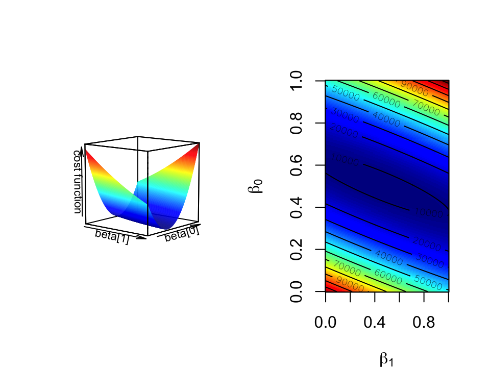
FIGURE 3.14: Cost function landscape for linear regression with changing beta values. The optimization process tries to find the lowest point in this landscape by implementing a strategy for updating beta values toward the lowest point in the landscape.
3.3.1.2 Not cost function but maximum likelihood function
We can also think of this problem from a more statistical point of view. In essence, we are looking for best statistical parameters, in this case \(\beta\) values, for our model that are most likely to produce such a scatter of data points given the explanatory variables. This is called the “maximum likelihood” approach. The approach assumes that a given response variable \(y_i\) follows a normal distribution with mean \(\beta_0+\beta_1x_i\) and variance \(s^2\). Therefore the probability of observing any given \(y_i\) value is dependent on the \(\beta_0\) and \(\beta_1\) values. Since \(x_i\), the explanatory variable, is fixed within our data set, we can maximize the probability of observing any given \(y_i\) by varying \(\beta_0\) and \(\beta_1\) values. The trick is to find \(\beta_0\) and \(\beta_1\) values that maximizes the probability of observing all the response variables in the dataset given the explanatory variables. The probability of observing a response variable \(y_i\) with assumptions we described above is shown below. Note that this assumes variance is constant and \(s^2=\frac{\sum{\epsilon_i}}{n-2}\) is an unbiased estimation for population variance, \(\sigma^2\).
\[P(y_{i})=\frac{1}{s\sqrt{2\pi} }e^{-\frac{1}{2}\left(\frac{y_i-(\beta_0 + \beta_1x_i)}{s}\right)^2}\]
Following from the probability equation above, the likelihood function (shown as \(L\) below) for linear regression is multiplication of \(P(y_{i})\) for all data points.
\[L=P(y_1)P(y_2)P(y_3)..P(y_n)=\prod\limits_{i=1}^n{P_i}\]
This can be simplified to the following equation by some algebra, assumption of normal distribution, and taking logs (since it is easier to add than multiply).
\[ln(L) = -nln(s\sqrt{2\pi}) - \frac{1}{2s^2} \sum\limits_{i=1}^n{(y_i-(\beta_0 + \beta_1x_i))^2} \]
As you can see, the right part of the function is the negative of the cost function defined above. If we wanted to optimize this function we would need to take the derivative of the function with respect to the \(\beta\) parameters. That means we can ignore the first part since there are no \(\beta\) terms there. This simply reduces to the negative of the cost function. Hence, this approach produces exactly the same result as the cost function approach. The difference is that we defined our problem within the domain of statistics. This particular function has still to be optimized. This can be done with some calculus without the need for an iterative approach.
The maximum likelihood approach also opens up other possibilities for regression. For the case above, we assumed that the points around the mean are distributed by normal distribution. However, there are other cases where this assumption may not hold. For example, for the count data the mean and variance relationship is not constant; the higher the mean counts, the higher the variance. In these cases, the regression framework with maximum likelihood estimation can still be used. We simply change the underlying assumptions about the distribution and calculate the likelihood with a new distribution in mind, and maximize the parameters for that likelihood. This gives way to “generalized linear model” approach where errors for the response variables can have other distributions than normal distribution. We will see examples of these generalized linear models in Chapter 8 and 10.
3.3.1.3 Linear algebra and closed-form solution to linear regression
The last approach we will describe is the minimization process using linear algebra. If you find this concept challenging, feel free to skip it, but scientific publications and other books frequently use matrix notation and linear algebra to define and solve regression problems. In this case, we do not use an iterative approach. Instead, we will minimize the cost function by explicitly taking its derivatives with respect to \(\beta\)’s and setting them to zero. This is doable by employing linear algebra and matrix calculus. This approach is also called “ordinary least squares”. We will not show the whole derivation here, but the following expression is what we are trying to minimize in matrix notation, which is basically a different notation of the same minimization problem defined above. Remember \(\epsilon_i=Y_i-(\beta_0+\beta_1x_i)\)
\[ \begin{aligned} \sum\epsilon_{i}^2=\epsilon^T\epsilon=(Y-{\beta}{X})^T(Y-{\beta}{X}) \\ =Y^T{Y}-2{\beta}^T{Y}+{\beta}^TX^TX{\beta} \end{aligned} \] After rearranging the terms, we take the derivative of \(\epsilon^T\epsilon\) with respect to \(\beta\), and equalize that to zero. We then arrive at the following for estimated \(\beta\) values, \(\hat{\beta}\):
\[\hat{\beta}=(X^TX)^{-1}X^TY\]
This requires you to calculate the inverse of the \(X^TX\) term, which could be slow for large matrices. Using an iterative approach over the cost function derivatives will be faster for larger problems. The linear algebra notation is something you will see in the papers or other resources often. If you input the data matrix X and solve the \((X^TX)^{-1}\) , you get the following values for \(\beta_0\) and \(\beta_1\) for simple regression . However, we should note that this simple linear regression case can easily be solved algebraically without the need for matrix operations. This can be done by taking the derivative of \(\sum{(y_i-(\beta_0+\beta_1x_i))^2}\) with respect to \(\beta_1\), rearranging the terms and equalizing the derivative to zero.
\[\hat{\beta_1}=\frac{\sum{(x_i-\overline{X})(y_i-\overline{Y})}}{ \sum{(x_i-\overline{X})^2} }\] \[\hat{\beta_0}=\overline{Y}-\hat{\beta_1}\overline{X}\]
3.3.1.4 Fitting lines in R
After all this theory, you will be surprised how easy it is to fit lines in R.
This is achieved just by the lm() function, which stands for linear models. Let’s do this
for a simulated data set and plot the fit. The first step is to simulate the
data. We will decide on \(\beta_0\) and \(\beta_1\) values. Then we will decide
on the variance parameter, \(\sigma\), to be used in simulation of error terms,
\(\epsilon\). We will first find \(Y\) values, just using the linear equation
\(Y=\beta0+\beta_1X\), for
a set of \(X\) values. Then, we will add the error terms to get our simulated values.
# set random number seed, so that the random numbers from the text
# is the same when you run the code.
set.seed(32)

# get 50 X values between 1 and 100
x = runif(50,1,100)

# set b0,b1 and variance (sigma)
b0 = 10
b1 = 2
sigma = 20
# simulate error terms from normal distribution
eps = rnorm(50,0,sigma)
# get y values from the linear equation and addition of error terms
y = b0 + b1*x+ eps
Now let us fit a line using the lm() function. The function requires a formula, and
optionally a data frame. We need to pass the following expression within the
lm() function, y~x, where y is the simulated \(Y\) values and x is the explanatory variables \(X\). We will then use the abline() function to draw the fit. The resulting plot is shown in Figure 3.15.
mod1=lm(y~x)

# plot the data points
plot(x,y,pch=20,
     ylab="Gene Expression",xlab="Histone modification score")
# plot the linear fit
abline(mod1,col="blue")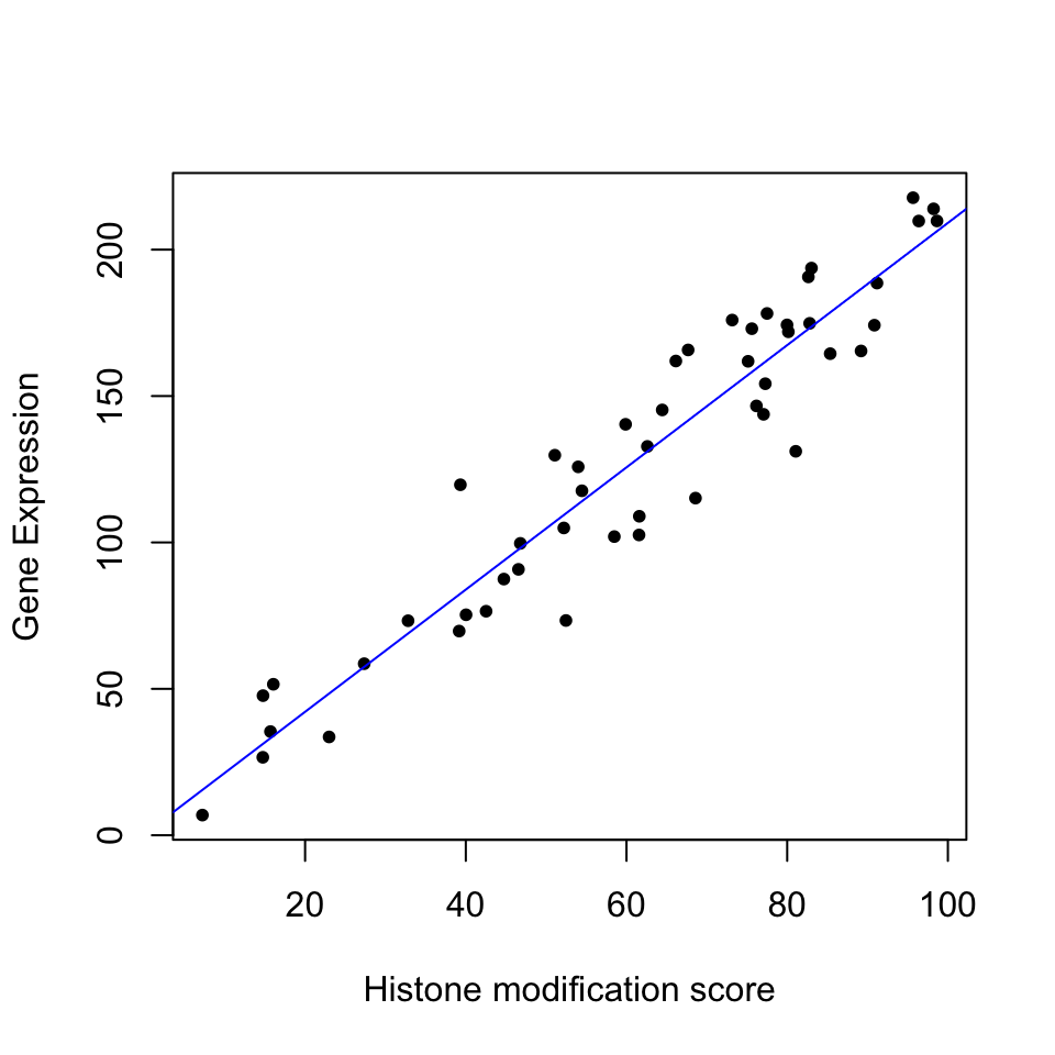
FIGURE 3.15: Gene expression and histone modification score modeled by linear regression.
3.3.2 How to estimate the error of the coefficients
Since we are using a sample to estimate the coefficients, they are not exact; with every random sample they will vary. In Figure 3.16, we take multiple samples from the population and fit lines to each sample; with each sample the lines slightly change. We are overlaying the points and the lines for each sample on top of the other samples. When we take 200 samples and fit lines for each of them, the line fits are variable. And, we get a normal-like distribution of \(\beta\) values with a defined mean and standard deviation, which is called standard error of the coefficients.
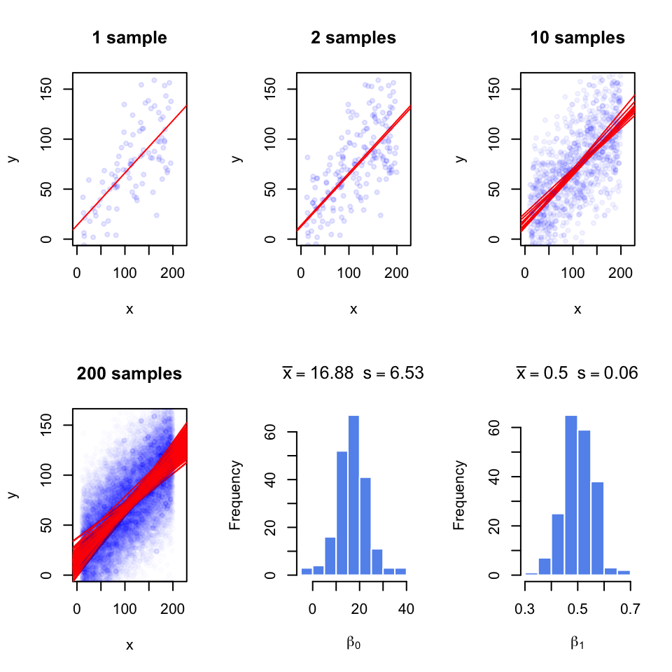
FIGURE 3.16: Regression coefficients vary with every random sample. The figure illustrates the variability of regression coefficients when regression is done using a sample of data points. Histograms depict this variability for \(b_0\) and \(b_1\) coefficients.
Normally, we will not have access to the population to do repeated sampling, model fitting, and estimation of the standard error for the coefficients. But there is statistical theory that helps us infer the population properties from the sample. When we assume that error terms have constant variance and mean zero , we can model the uncertainty in the regression coefficients, \(\beta\)s. The estimates for standard errors of \(\beta\)s for simple regression are as follows and shown without derivation.
\[ \begin{aligned} s=RSE=\sqrt{\frac{\sum{(y_i-(\beta_0+\beta_1x_i))^2}}{n-2} } =\sqrt{\frac{\sum{\epsilon^2}}{n-2} } \\ SE(\hat{\beta_1})=\frac{s}{\sqrt{\sum{(x_i-\overline{X})^2}}} \\ SE(\hat{\beta_0})=s\sqrt{ \frac{1}{n} + \frac{\overline{X}^2}{\sum{(x_i-\overline{X})^2} } } \end{aligned} \]
Notice that that \(SE(\beta_1)\) depends on the estimate of variance of residuals shown as \(s\) or Residual Standard Error (RSE). Notice also the standard error depends on the spread of \(X\). If \(X\) values have more variation, the standard error will be lower. This intuitively makes sense since if the spread of \(X\) is low, the regression line will be able to wiggle more compared to a regression line that is fit to the same number of points but covers a greater range on the X-axis.
The standard error estimates can also be used to calculate confidence intervals and test hypotheses, since the following quantity, called t-score, approximately follows a t-distribution with \(n-p\) degrees of freedom, where \(n\) is the number of data points and \(p\) is the number of coefficients estimated.
\[ \frac{\hat{\beta_i}-\beta_test}{SE(\hat{\beta_i})}\]
Often, we would like to test the null hypothesis if a coefficient is equal to zero or not. For simple regression, this could mean if there is a relationship between the explanatory variable and the response variable. We would calculate the t-score as follows \(\frac{\hat{\beta_i}-0}{SE(\hat{\beta_i})}\), and compare it to the t-distribution with \(d.f.=n-p\) to get the p-value.
We can also calculate the uncertainty of the regression coefficients using confidence intervals, the range of values that are likely to contain \(\beta_i\). The 95% confidence interval for \(\hat{\beta_i}\) is \(\hat{\beta_i}\) ± \(t_{0.975}SE(\hat{\beta_i})\). \(t_{0.975}\) is the 97.5% percentile of the t-distribution with \(d.f. = n – p\).
In R, the summary() function will test all the coefficients for the null hypothesis
\(\beta_i=0\). The function takes the model output obtained from the lm()
function. To demonstrate this, let us first get some data. The procedure below
simulates data to be used in a regression setting and it is useful to examine
what the linear model expects to model the data.
Since we have the data, we can build our model and call the summary function.
We will then use the confint() function to get the confidence intervals on the
coefficients and the coef() function to pull out the estimated coefficients from
the model.
##
## Call:
## lm(formula = y ~ x)
##
## Residuals:
##    Min     1Q Median     3Q    Max
## -77.11 -18.44   0.33  16.06  57.23
##
## Coefficients:
##             Estimate Std. Error t value Pr(>|t|)
## (Intercept) 13.24538    6.28869   2.106   0.0377 *
## x            0.49954    0.05131   9.736 4.54e-16 ***
## ---
## Signif. codes:  0 '***' 0.001 '**' 0.01 '*' 0.05 '.' 0.1 ' ' 1
##
## Residual standard error: 28.77 on 98 degrees of freedom
## Multiple R-squared:  0.4917, Adjusted R-squared:  0.4865
## F-statistic: 94.78 on 1 and 98 DF, p-value: 4.537e-16## 2.5 % 97.5 %
## (Intercept) 0.7656777 25.7250883
## x 0.3977129 0.6013594## (Intercept) x
## 13.2453830 0.4995361The summary() function prints out an extensive list of values.
The “Coefficients” section has the estimates, their standard error, t score,
and the p-value from the hypothesis test \(H_0:\beta_i=0\). As you can see, the
estimate we get for the coefficients and their standard errors are close to
the ones we get from repeatedly sampling and getting a distribution of
coefficients. This is statistical inference at work, so we can estimate the
population properties within a certain error using just a sample.
3.3.3 Accuracy of the model
If you have observed the table output of the summary() function, you must have noticed there are some other outputs, such as “Residual standard error”,
“Multiple R-squared” and “F-statistic”. These are metrics that are useful
for assessing the accuracy of the model. We will explain them one by one.
RSE is simply the square-root of the sum of squared error terms, divided by degrees of freedom, \(n-p\). For the simple linear regression case, degrees of freedom is \(n-2\). Sum of the squares of the error terms is also called the “Residual sum of squares”, RSS. So the RSE is calculated as follows:
\[ s=RSE=\sqrt{\frac{\sum{(y_i-\hat{Y_i})^2 }}{n-p}}=\sqrt{\frac{RSS}{n-p}}\]
The RSE is a way of assessing the model fit. The larger the RSE the worse the model is. However, this is an absolute measure in the units of \(Y\) and we have nothing to compare against. One idea is that we divide it by the RSS of a simpler model for comparative purposes. That simpler model is in this case is the model with the intercept, \(\beta_0\). A very bad model will have close to zero coefficients for explanatory variables, and the RSS of that model will be close to the RSS of the model with only the intercept. In such a model the intercept will be equal to \(\overline{Y}\). As it turns out, the RSS of the model with just the intercept is called the “Total Sum of Squares” or TSS. A good model will have a low \(RSS/TSS\). The metric \(R^2\) uses these quantities to calculate a score between 0 and 1, and the closer to 1, the better the model. Here is how it is calculated:
\[R^2=1-\frac{RSS}{TSS}=\frac{TSS-RSS}{TSS}=1-\frac{RSS}{TSS}\]
The \(TSS-RSS\) part of the formula is often referred to as “explained variability” in
the model. The bottom part is for “total variability”. With this interpretation, the higher
the “explained variability”, the better the model. For simple linear regression
with one explanatory variable, the square root of \(R^2\) is a quantity known
as the absolute value of the correlation coefficient, which can be calculated for any pair of variables, not only
the
response and the explanatory variables. Correlation is the general measure of
linear
relationship between two variables. One
of the most popular flavors of correlation is the Pearson correlation coefficient. Formally, it is the
covariance of X and Y divided by multiplication of standard deviations of
X and Y. In R, it can be calculated with the cor() function.
\[ r_{xy}=\frac{cov(X,Y)}{\sigma_x\sigma_y} =\frac{\sum\limits_{i=1}^n (x_i-\bar{x})(y_i-\bar{y})} {\sqrt{\sum\limits_{i=1}^n (x_i-\bar{x})^2 \sum\limits_{i=1}^n (y_i-\bar{y})^2}} \] In the equation above, \(cov\) is the covariance; this is again a measure of how much two variables change together, like correlation. If two variables show similar behavior, they will usually have a positive covariance value. If they have opposite behavior, the covariance will have a negative value. However, these values are boundless. A normalized way of looking at covariance is to divide covariance by the multiplication of standard errors of X and Y. This bounds the values to -1 and 1, and as mentioned above, is called Pearson correlation coefficient. The values that change in a similar manner will have a positive coefficient, the values that change in an opposite manner will have a negative coefficient, and pairs that do not have a linear relationship will have \(0\) or near \(0\) correlation. In Figure 3.17, we are showing \(R^2\), the correlation coefficient, and covariance for different scatter plots.
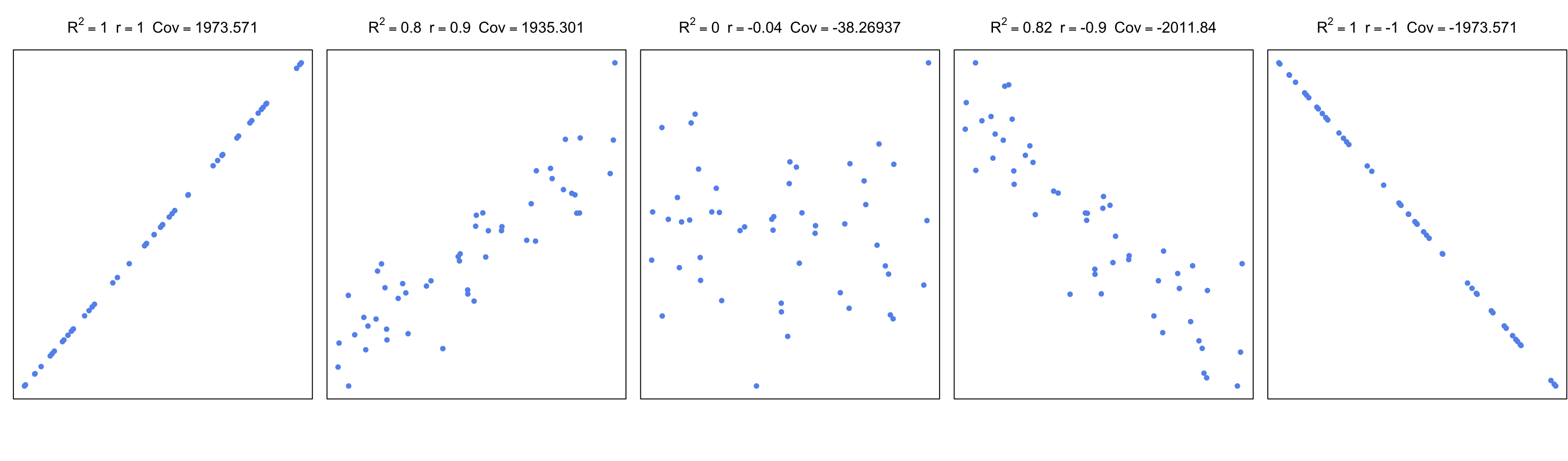
FIGURE 3.17: Correlation and covariance for different scatter plots.
For simple linear regression, correlation can be used to assess the model. However, this becomes useless as a measure of general accuracy if there is more than one explanatory variable as in multiple linear regression. In that case, \(R^2\) is a measure of accuracy for the model. Interestingly, the square of the correlation of predicted values and original response variables (\((cor(Y,\hat{Y}))^2\) ) equals \(R^2\) for multiple linear regression.
The last accuracy measure, or the model fit in general we are going to explain is F-statistic. This is a quantity that depends on the RSS and TSS again. It can also answer one important question that other metrics cannot easily answer. That question is whether or not any of the explanatory variables have predictive value or in other words if all the explanatory variables are zero. We can write the null hypothesis as follows:
\[H_0: \beta_1=\beta_2=\beta_3=...=\beta_p=0 \]
where the alternative is:
\[H_1: \text{at least one } \beta_i \neq 0 \]
Remember that \(TSS-RSS\) is analogous to “explained variability” and the RSS is analogous to “unexplained variability”. For the F-statistic, we divide explained variance by unexplained variance. Explained variance is just the \(TSS-RSS\) divided by degrees of freedom, and unexplained variance is the RSE. The ratio will follow the F-distribution with two parameters, the degrees of freedom for the explained variance and the degrees of freedom for the unexplained variance. The F-statistic for a linear model is calculated as follows.
\[F=\frac{(TSS-RSS)/(p-1)}{RSS/(n-p)}=\frac{(TSS-RSS)/(p-1)}{RSE} \sim F(p-1,n-p)\]
If the variances are the same, the ratio will be 1, and when \(H_0\) is true, then
it can be shown that expected value of \((TSS-RSS)/(p-1)\) will be \(\sigma^2\), which is estimated by the RSE. So, if the variances are significantly different,
the ratio will need to be significantly bigger than 1.
If the ratio is large enough we can reject the null hypothesis. To assess that,
we need to use software or look up the tables for F statistics with calculated
parameters. In R, function qf() can be used to calculate critical value of the
ratio. Benefit of the F-test over
looking at significance of coefficients one by one is that we circumvent
multiple testing problem. If there are lots of explanatory variables
at least 5% of the time (assuming we use 0.05 as P-value significance
cutoff), p-values from coefficient t-tests will be wrong. In summary, F-test is a better choice for testing if there is any association
between the explanatory variables and the response variable.
3.3.4 Regression with categorical variables
An important feature of linear regression is that categorical variables can be used as explanatory variables, this feature is very useful in genomics where explanatory variables can often be categorical. To put it in context, in our histone modification example we can also include if promoters have CpG islands or not as a variable. In addition, in differential gene expression, we usually test the difference between different conditions, which can be encoded as categorical variables in a linear regression. We can sure use the t-test for that as well if there are only 2 conditions, but if there are more conditions and other variables to control for, such as age or sex of the samples, we need to take those into account for our statistics, and the t-test alone cannot handle such complexity. In addition, when we have categorical variables we can also have numeric variables in the model and we certainly do not have to include only one type of variable in a model.
The simplest model with categorical variables includes two levels that can be encoded in 0 and 1. Below, we show linear regression with categorical variables. We then plot the fitted line. This plot is shown in Figure 3.18.
set.seed(100)
gene1=rnorm(30,mean=4,sd=2)
gene2=rnorm(30,mean=2,sd=2)
gene.df=data.frame(exp=c(gene1,gene2),
                  group=c( rep(1,30),rep(0,30) ) )

mod2=lm(exp~group,data=gene.df)
summary(mod2)
##
## Call:
## lm(formula = exp ~ group, data = gene.df)
##
## Residuals:
## Min 1Q Median 3Q Max
## -4.7290 -1.0664 0.0122 1.3840 4.5629
##
## Coefficients:
## Estimate Std. Error t value Pr(>|t|)
## (Intercept) 2.1851 0.3517 6.214 6.04e-08 ***
## group 1.8726 0.4973 3.765 0.000391 ***
## ---
## Signif. codes: 0 '***' 0.001 '**' 0.01 '*' 0.05 '.' 0.1 ' ' 1
##
## Residual standard error: 1.926 on 58 degrees of freedom
## Multiple R-squared: 0.1964, Adjusted R-squared: 0.1826
## F-statistic: 14.18 on 1 and 58 DF, p-value: 0.0003905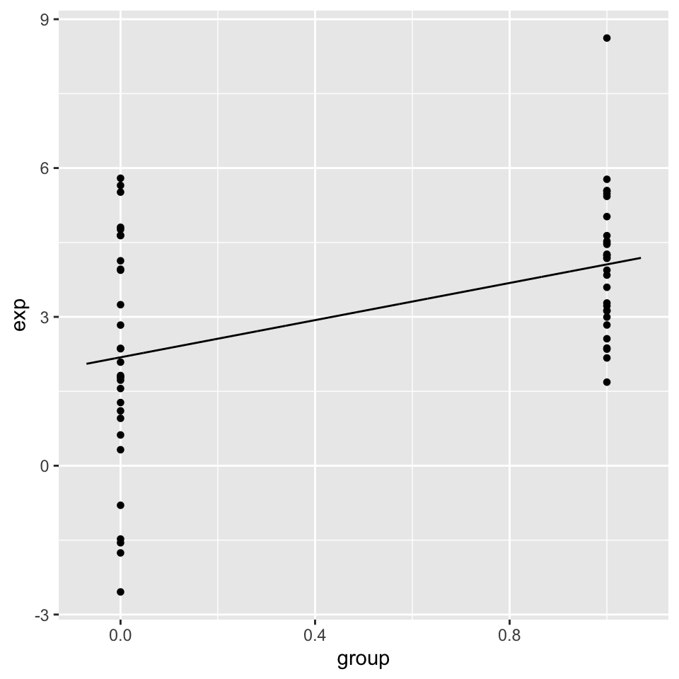
FIGURE 3.18: Linear model with a categorical variable coded as 0 and 1.
We can even compare more levels, and we do not even have to encode them
ourselves. We can pass categorical variables to the lm() function.
gene.df=data.frame(exp=c(gene1,gene2,gene2),
                  group=c( rep("A",30),rep("B",30),rep("C",30) )
                  )

mod3=lm(exp~group,data=gene.df)
summary(mod3)
##
## Call:
## lm(formula = exp ~ group, data = gene.df)
##
## Residuals:
## Min 1Q Median 3Q Max
## -4.7290 -1.0793 -0.0976 1.4844 4.5629
##
## Coefficients:
## Estimate Std. Error t value Pr(>|t|)
## (Intercept) 4.0577 0.3781 10.731 < 2e-16 ***
## groupB -1.8726 0.5348 -3.502 0.000732 ***
## groupC -1.8726 0.5348 -3.502 0.000732 ***
## ---
## Signif. codes: 0 '***' 0.001 '**' 0.01 '*' 0.05 '.' 0.1 ' ' 1
##
## Residual standard error: 2.071 on 87 degrees of freedom
## Multiple R-squared: 0.1582, Adjusted R-squared: 0.1388
## F-statistic: 8.174 on 2 and 87 DF, p-value: 0.00055823.3.5 Regression pitfalls
In most cases one should look at the error terms (residuals) vs. the fitted values plot. Any structure in this plot indicates problems such as non-linearity, correlation of error terms, non-constant variance or unusual values driving the fit. Below we briefly explain the potential issues with the linear regression.
3.3.5.0.1 Non-linearity
If the true relationship is far from linearity, prediction accuracy is reduced and all the other conclusions are questionable. In some cases, transforming the data with \(logX\), \(\sqrt{X}\), and \(X^2\) could resolve the issue.
3.3.5.0.2 Correlation of explanatory variables
If the explanatory variables are correlated that could lead to something
known as multicolinearity. When this happens SE estimates of the coefficients will be too large. This is usually observed in time-course
data.
3.3.5.0.3 Correlation of error terms
This assumes that the errors of the response variables are uncorrelated with each other. If they are, the confidence intervals of the coefficients might be too narrow.
3.3.5.0.4 Non-constant variance of error terms
This means that different response variables have the same variance in their errors, regardless of the values of the predictor variables. If the errors are not constant (ex: the errors grow as X values increase), this will result in unreliable estimates in standard errors as the model assumes constant variance. Transformation of data, such as \(logX\) and \(\sqrt{X}\), could help in some cases.
3.3.5.0.5 Outliers and high leverage points
Outliers are extreme values for Y and high leverage points are unusual X values. Both of these extremes have the power to affect the fitted line and the standard errors. In some cases (Ex: if there are measurement errors), they can be removed from the data for a better fit.
Want to know more ?
- Linear models and derivations of equations including matrix notation
- Applied Linear Statistical Models by Kutner, Nachtsheim, et al. (Kutner, Nachtsheim, and Neter 2003)
- Elements of Statistical Learning by Hastie & Tibshirani (J. Friedman, Hastie, and Tibshirani 2001)
- An Introduction to Statistical Learning by James, Witten, et al. (James, Witten, Hastie, et al. 2013)
References
Friedman, Hastie, and Tibshirani. 2001. The Elements of Statistical Learning. Vol. 1. Springer series in statistics New York.
James, Witten, Hastie, and Tibshirani. 2013. An Introduction to Statistical Learning: With Applications in R. Springer Texts in Statistics. Springer New York. https://books.google.de/books?id=qcI\_AAAAQBAJ.
Kutner, Nachtsheim, and Neter. 2003. Applied Linear Regression Models. The Mcgraw-Hill/Irwin Series Operations and Decision Sciences. McGraw-Hill Higher Education. https://books.google.de/books?id=0nAMAAAACAAJ.