11.5 Biological interpretation of latent factors

11.5.1 Inspection of feature weights in loading vectors

The most straightforward way to go about interpreting the latent factors in a biological context, is to look at the coefficients which are associated with them. The latent variable models introduced above all take the linear form \(X \approx WH\), where \(W\) is a factor matrix, with coefficients tying each latent variable with each of the features in the \(L\) original multi-omics data matrices. By inspecting these coefficients, we can get a sense of which multi-omics features are co-regulated. The code snippet below generates Figure 11.15, which shows the coefficients of the Joint NMF analysis above:

# create an annotation dataframe for the heatmap
# for each feature, indicating its omics-type
data_anno <- data.frame(
  omics=c(rep('expression',dim(x1)[1]),
          rep('mut',dim(x2)[1]),
          rep('cnv',dim(x3.featnorm.frobnorm.nonneg)[1])))
rownames(data_anno) <- c(rownames(x1),
                         paste0("mut:", rownames(x2)),
                         rownames(x3.featnorm.frobnorm.nonneg))
rownames(nmfw) <- rownames(data_anno)

# generate the heat map
pheatmap::pheatmap(nmfw,
                   cluster_cols = FALSE,
                   annotation_row = data_anno,
                   main="NMF coefficients",
                   clustering_distance_rows = "manhattan",
                   fontsize_row = 1)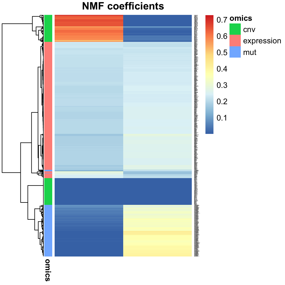

FIGURE 11.15: Heatmap showing the association of input features from multi-omics data (gene expression, copy number variation, and mutations), with JNMF factors. Gene expression features dominate both factors, but copy numbers and mutations mostly affect only one factor each.

Inspection of the factor coefficients in the heatmap above reveals that Joint NMF has found two nearly orthogonal non-negative factors. One is associated with high expression of the HOXC11, ZIC5, and XIRP1 genes, frequent mutations in the BRAF, PCDHGA6, and DNAH5 genes, as well as losses in the 18q12.2 and gains in 8p21.1 cytobands. The other factor is associated with high expression of the SOX1 gene, more frequent mutations in the APC, KRAS, and TP53 genes, and a weak association with some CNVs.

11.5.1.1 Disentangled representations

The property displayed above, where each feature is predominantly associated with only a single factor, is termed disentangledness, i.e. it leads to disentangled latent variable representations, as changing one input feature only affects a single latent variable. This property is very desirable as it greatly simplifies the biological interpretation of modules. Here, we have two modules with a set of co-occurring molecular signatures which merit deeper investigation into the mechanisms by which these different omics features are related. For this reason, NMF is widely used in computational biology today.

11.5.2 Making sense of factors using enrichment analysis

In order to investigate the oncogenic processes that drive the differences between tumors, we may draw upon biological prior knowledge by looking for overlaps between genes that drive certain tumors, and genes involved in familiar biological processes.

11.5.2.1 Enrichment analysis

The recent decades of genomics have uncovered many of the ways in which genes cooperate to perform biological functions in concert. This work has resulted in rich annotations of genes, groups of genes, and the different functions they carry out. Examples of such annotations include the Gene Ontology Consortium’s GO terms (Ashburner, Ball, Blake, et al. 2000, @go_latest_paper), the Reactome pathways database (A. Fabregat, Jupe, Matthews, et al. 2018), and the Kyoto Encyclopaedia of Genes and Genomes (Kanehisa, Furumichi, Tanabe, et al. 2017). These resources, as well as others, publish lists of so-called gene sets, or pathways, which are sets of genes which are known to operate together in some biological function, e.g. protein synthesis, DNA mismatch repair, cellular adhesion, and many other functions. Gene set enrichment analysis is a method which looks for overlaps between genes which we have found to be of interest, e.g. by them being implicated in a certain tumor type, and the a-priori gene sets discussed above.

In the context of making sense of latent factors, the question we will be asking is whether the genes which drive the value of a latent factor (the genes with the highest factor coefficients) also belong to any interesting annotated gene sets, and whether the overlap is greater than we would expect by chance. If there are \(N\) genes in total, \(K\) of which belong to a gene set, the probability that \(k\) out of the \(n\) genes associated with a latent factor are also associated with a gene set is given by the hypergeometric distribution:

\[ P(k) = \frac{{\binom{K}{k}} - \binom{N-K}{n-k}}{\binom{N}{n}}. \]

The hypergeometric test uses the hypergeometric distribution to assess the statistical significance of the presence of genes belonging to a gene set in the latent factor. The null hypothesis is that there is no relationship between genes in a gene set, and genes in a latent factor. When testing for over-representation of gene set genes in a latent factor, the P value from the hypergeometric test is the probability of getting \(k\) or more genes from a gene set in a latent factor

\[ p = \sum_{i=k}^K P(k=i). \]

The hypergeometric enrichment test is also referred to as Fisher’s one-sided exact test. This way, we can determine if the genes associated with a factor significantly overlap (beyond chance) the genes involved in a biological process. Because we will typically be testing many gene sets, we will also need to apply multiple testing correction, such as Benjamini-Hochberg correction (see Chapter 3, multiple testing correction).

11.5.2.2 Example in R

In R, we can do this analysis using the enrichR package, which gives us access to many gene set libraries. In the example below, we will find the genes associated with preferentially NMF factor 1 or NMF factor 2, by the contribution of those genes’ expression values to the factor. Then, we’ll use enrichR to query the Gene Ontology terms which might be overlapping:

require(enrichR)

# select genes associated preferentially with each factor
# by their relative loading in the W matrix
genes.factor.1 <- names(which(nmfw[1:dim(x1)[1],1] > nmfw[1:dim(x1)[1],2]))
genes.factor.2 <- names(which(nmfw[1:dim(x1)[1],1] < nmfw[1:dim(x1)[1],2]))

# call the enrichr function to find gene sets enriched
# in each latent factor in the GO Biological Processes 2018 library
go.factor.1 <- enrichR::enrichr(genes.factor.1,
                                databases = c("GO_Biological_Process_2018")
                                )$GO_Biological_Process_2018
go.factor.2 <- enrichR::enrichr(genes.factor.2,
                                databases = c("GO_Biological_Process_2018")
                                )$GO_Biological_Process_2018

The top GO terms associated with NMF factor 2 are shown in Table ??:

11.5.3 Interpretation using additional covariates

Another way to ascribe biological significance to the latent variables is by correlating them with additional covariates we might have about the samples. In our example, the colorectal cancer tumors have also been characterized for microsatellite instability (MSI) status, using an external test (typically PCR-based). By examining the latent variable values as they relate to a tumor’s MSI status, we might discover that we’ve learned latent factors that are related to it. The following code snippet demonstrates how this might be looked into, by generating Figures 11.16 and 11.17:

# create a data frame holding covariates (age, gender, MSI status)
a <- data.frame(age=covariates$age,
                gender=as.numeric(covariates$gender),
                msi=covariates$msi)

## Warning in data.frame(age = covariates$age, gender =
## as.numeric(covariates$gender), : NAs introduced by coercion

b <- nmf.h
colnames(b) <- c('factor1', 'factor2')

# concatenate the covariate dataframe with the H matrix
cov_factor <- cbind(a,b)

# generate the figure
ggplot2::ggplot(cov_factor, ggplot2::aes(x=msi, y=factor1, group=msi)) +
  ggplot2::geom_boxplot() +
  ggplot2::ggtitle("NMF factor 1 microsatellite instability")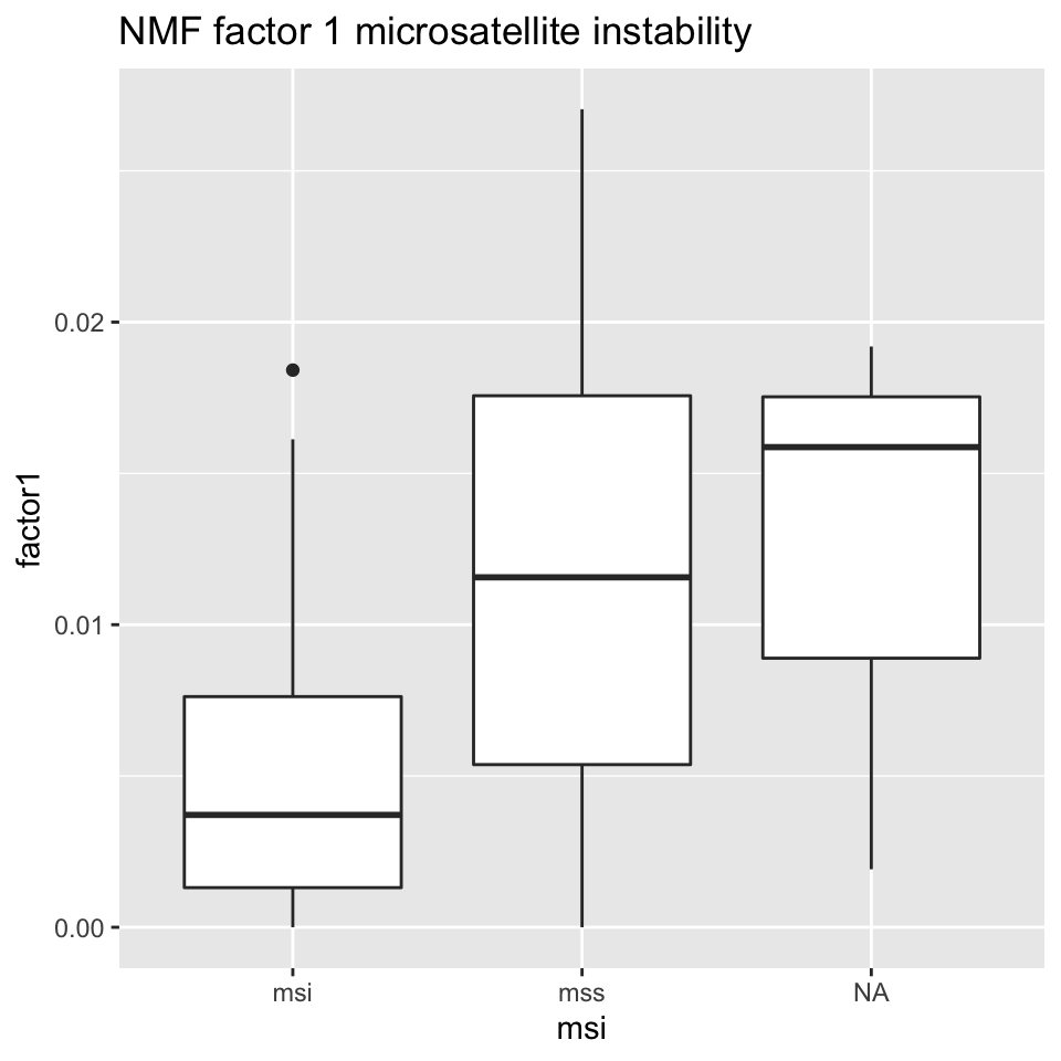

FIGURE 11.16: Box plot showing MSI/MSS status distribution and NMF factor 1 values.

ggplot2::ggplot(cov_factor, ggplot2::aes(x=msi, y=factor2, group=msi)) +
  ggplot2::geom_boxplot() +
  ggplot2::ggtitle("NMF factor 2 and microsatellite instability")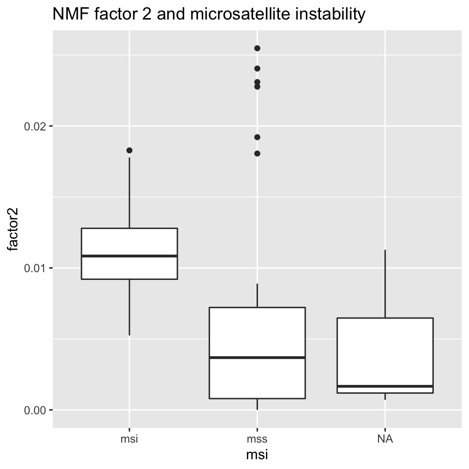

FIGURE 11.17: Box plot showing MSI/MSS status distribution and NMF factor 2 values.

Figures 11.16 and 11.17 show that NMF factor 1 and NMF factor 2 are separated by the MSI or MSS (microsatellite stability) status of the tumors.

References

Ashburner, Ball, Blake, et al. 2000. “Gene ontology: tool for the unification of biology. The Gene Ontology Consortium.” Nat. Genet. 25 (1): 25–29.

Fabregat, Jupe, Matthews, et al. 2018. “The Reactome Pathway Knowledgebase.” Nucleic Acids Res. 46 (D1): D649–D655.

Kanehisa, Furumichi, Tanabe, Sato, and Morishima. 2017. “KEGG: new perspectives on genomes, pathways, diseases and drugs.” Nucleic Acids Res. 45 (D1): D353–D361.