5.14 Other supervised algorithms

We will next introduce a couple of other supervised algorithms for completeness but in less detail. These algorithms are also as popular as the others we introduced above and people who are interested in computational genomics see them used in the field for different problems. These algorithms also fit to the general framework of optimization of a cost/loss function. However, the approaches to the construction of the cost function and the cost function itself are different in each case.

5.14.1 Gradient boosting

Gradient boosting is a prediction model that uses an ensemble of decision trees similar to random forest. However, the decision trees are added sequentially, which is why these models are also called “Multiple Additive Regression Trees (MART)” (Friedman and Meulman 2003). Apart from this, you will see similar methods called “Gradient boosting machines (GBM)”(J. H. Friedman 2001) or “Boosted regression trees (BRT)” (Elith, Leathwick, and Hastie 2008) in the literature.

Generally, “boosting” refers to an iterative learning approach where each new model tries to focus on data points where the previous ensemble of simple models did not predict well. Gradient boosting is an improvement over that, where each new model tries to focus on the residual errors (prediction error for the current ensemble of models) of the previous model. Specifically in gradient boosting, the simple models are trees. As in random forests, many trees are grown but in this case, trees are sequentially grown and each tree focuses on fixing the shortcomings of the previous trees. Figure 5.13 shows this concept. One of the most widely used algorithms for gradient boosting is XGboost which stands for “extreme gradient boosting” (Chen and Guestrin 2016). Below we will demonstrate how to use this on our problem. XGboost as well as other gradient boosting methods has many parameters to regularize and optimize the complexity of the model. Finding the best parameters for your problem might take some time. However, this flexibility comes with benefits; methods depending on XGboost have won many machine learning competitions (Chen and Guestrin 2016).

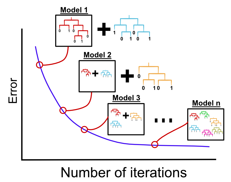
Gradient boosting machines concept. Individual decision trees are built sequentially in order to fix the errors from the previous trees.

FIGURE 5.13: Gradient boosting machines concept. Individual decision trees are built sequentially in order to fix the errors from the previous trees.

The most important parameters are number of trees (nrounds), tree depth (max_depth), and learning rate or shrinkage (eta). Generally, the more trees we have, the better the algorithm will learn because each tree tries to fix classification errors that the previous tree ensemble could not perform. Having too many trees might cause overfitting. However, the learning rate parameter, eta, combats that by shrinking the contribution of each new tree. This can be set to lower values if you have many trees. You can either set a large number of trees and then tune the model with the learning rate parameter or set the learning rate low, say to \(0.01\) or \(0.1\) and tune the number of trees. Similarly, tree depth also controls for overfitting. The deeper the tree, the more usually it will overfit. This has to be tuned as well; the default is at 6. You can try to explore a range around the default. Apart from these, as in random forests, you can subsample the training data and/or the predictive variables. These strategies can also help you counter overfitting.

We are now going to use XGboost with the caret package on our cancer subtype classification problem. We are going to try different learning rate parameters. In this instance, we also subsample the dataset before we train each tree. The “subsample” parameter controls this and we set this to be 0.5, which means that before we train a tree we will sample 50% of the data and use only that portion to train the tree.

library(xgboost)
set.seed(17)

# we will just set up 5-fold cross validation
trctrl <- trainControl(method = "cv",number=5)

# we will now train elastic net model
# it will try
gbFit <- train(subtype~., data = training, 
                 method = "xgbTree",
                 trControl=trctrl,
                 # paramters to try
                 tuneGrid = data.frame(nrounds=200,
                                       eta=c(0.05,0.1,0.3),
                                       max_depth=4,
                                       gamma=0,
                                       colsample_bytree=1,
                                       subsample=0.5,
                                       min_child_weight=1))
                                       

# best parameters by cross-validation accuracy
gbFit$bestTune

##   nrounds max_depth eta gamma colsample_bytree min_child_weight subsample
## 2     200         4 0.1     0                1                1       0.5

Similar to random forests, we can estimate the variable importance for gradient boosting using the improvement in gini impurity or other performance-related metrics every time a variable is selected in a tree. Again, the caret::varImp() function can be used to plot the importance metrics.

Want to know more ?

More background on gradient boosting and XGboost: (https://xgboost.readthedocs.io/en/latest/tutorials/model.html). This explains the cost/loss function and regularization in more detail.
Lecture on Gradient boosting and random forests by Trevor Hastie: (https://youtu.be/wPqtzj5VZus)

5.14.2 Support Vector Machines (SVM)

Support vector machines (SVM) were popularized in the 90s due the efficiency and the performance of the algorithm (Boser, Guyon, and Vapnik 1992). The algorithm works by identifying the optimal decision boundary that separates the data points into different groups (or classes), and then predicts the class of new observations based on this separation boundary. Depending on the situation, the different groups might be separable by a linear straight line or by a non-linear boundary line or plane. If you review k-NN decision boundaries in Figure 5.7, you can see that the decision boundary is not linear. SVM can deal with linear or non-linear decision boundaries.

First, SVM can map the data to higher dimensions where the decision boundary can be linear. This is achieved by applying certain mathematical functions, called “kernel functions”, to the predictor variable space. For example, a second-degree polynomial can be applied to predictor variables which creates new variables and in this new space the problem is linearly separable. Figure 5.14 demonstrates this concept where points in feature space are mapped to quadratic space where linear separation is possible.

Support vector machine concept. With the help of a kernel function,points in feature space are mapped to higher dimensions where linear separation is possible.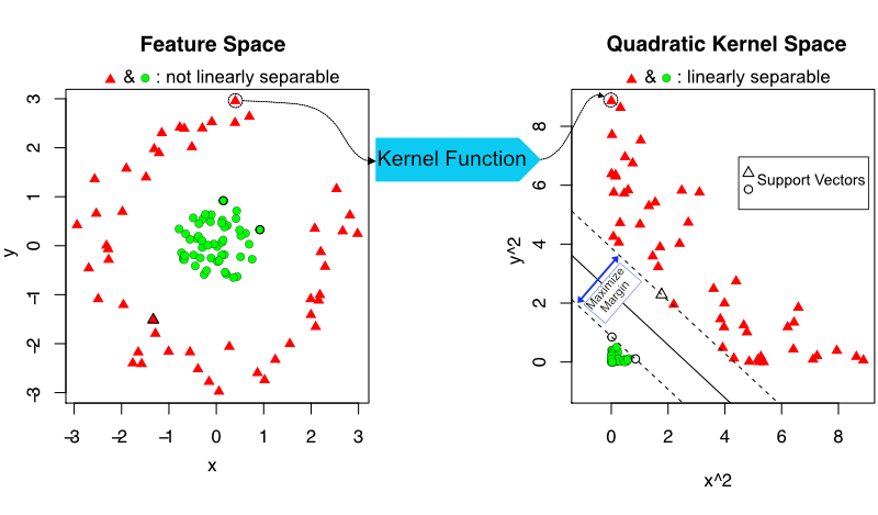

FIGURE 5.14: Support vector machine concept. With the help of a kernel function,points in feature space are mapped to higher dimensions where linear separation is possible.

Second, SVM not only tries to find a decision boundary, but tries to find the boundary with the largest buffer zone on the sides of the boundary. Having a boundary with a large buffer or “margin”, as it is formally called, will perform better for the new data points not used in the model training (margin is marked in Figure 5.14 ). In addition, SVM calculates the decision boundary with some error toleration. As we have seen it may not always be possible to find a linear boundary that perfectly separates the classes. SVM tolerates some degree of error, as in data points on the wrong side of the decision boundary.

Another important feature of the algorithm is that SVM decides on the decision boundary by only relying on the “landmark” data points, formally known as “support vectors”. These are points that are closest to the decision boundary and harder to classify. By keeping track of such points only for decision boundary creation, the computational complexity of the algorithm is reduced. However, this depends on the margin or the buffer zone. If we have a large margin then there are many landmark points. The extent of the margin is also related to the variance-bias trade-off. If the allowed margin is small the classification will try to find a boundary that makes fewer errors in the training set therefore might overfit. If the margin is larger, it will tolerate more errors in the training set and might generalize better. Practically, this is controlled by the “C” or “Cost” parameter in the SVM example we will show below. Another important choice we will make is the kernel function. Below we use the radial basis kernel function. This function provides an extra predictor dimension where the problem is linearly separable. The model we will use has only one parameter, which is “C”. It is recommended that \(C\) is in the form of \(2^k\) where \(k\) is in the range of -5 and 15 (Hsu, Chang, Lin, et al. 2003). Another parameter that can be tuned is related to the radial basis function called “sigma”. A smaller sigma means less bias and more variance, while a larger sigma means less variance and more bias. Again, exponential sequences are recommended for tuning that (Hsu, Chang, Lin, et al. 2003). We will set it to 1 for demonstration purposes below.

#svm code here
library(kernlab)
set.seed(17)

# we will just set up 5-fold cross validation
trctrl <- trainControl(method = "cv",number=5)

# we will now train elastic net model
# it will try
svmFit <- train(subtype~., data = training, 
                # this SVM used radial basis function
                 method = "svmRadial", 
                 trControl=trctrl,
                tuneGrid=data.frame(C=c(0.25,0.5,1),
                                    sigma=1))

Want to know more ?

MIT lecture by Patrick Winston on SVM: https://youtu.be/_PwhiWxHK8o. This lecture explains the concept with some mathematical background. It is not hard to follow. You should be able to follow this if you know what vectors are and if you have some knowledge on derivatives and basic algebra.
Online demo for SVM: (https://cs.stanford.edu/people/karpathy/svmjs/demo/). You can play with sigma and C parameters for radial basis SVM and see how they affect the decision boundary.

5.14.3 Neural networks and deep versions of it

Neural networks are another popular machine learning method which is recently regaining popularity. The earlier versions of the algorithm were popularized in the 80s and 90s. The advantage of neural networks is like SVM, they can model non-linear decision boundaries. The basic idea of neural networks is to combine the predictor variables in order to model the response variable as a non-linear function. In a neural network, input variables pass through several layers that combine the variables and transform those combinations and recombine outputs depending on how many layers the network has. In the conceptual example in Figure 5.15 the input nodes receive predictor variables and make linear combinations of them in the form of \(\sum ( w_ixi +b)\). Simply put, the variables are multiplied with weights and summed up. This is what we call “linear combination”. These quantities are further fed into another layer called the hidden layer where an activation function is applied on the sums. And these results are further fed into an output node which outputs class probabilities assuming we are working on a classification algorithm. There could be many more hidden layers that will even further combine the output from hidden layers before them. The algorithm in the end also has a cost function similar to the logistic regression cost function, but it now has to estimate all the weight parameters: \(w_i\). This is a more complicated problem than logistic regression because of the number of parameters to be estimated but neural networks are able to fit complex functions due their parameter space flexibility as well.

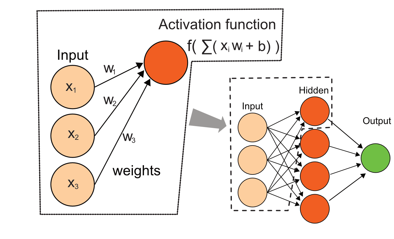
Diagram for a simple neural network, their combinations pass through hidden layers and are combined again for the output. Predictor variables are fed to the network and weights are adjusted to optimize the cost function.

FIGURE 5.15: Diagram for a simple neural network, their combinations pass through hidden layers and are combined again for the output. Predictor variables are fed to the network and weights are adjusted to optimize the cost function.

In a practical sense, the number of nodes in the hidden layer (size) and some regularization on the weights can be applied to control for overfitting. This is called the calculated (decay) parameter controls for overfitting.

We will train a simple neural network on our cancer data set. In this simple example, the network architecture is somewhat fixed. We can only the choose number of nodes (denoted by “size”) in the hidden layer and a regularization parameter (denoted by “decay”). Increasing the number of nodes in the hidden layer or in other implementations increasing the number of the hidden layers, will help model non-linear relationships but can overfit. One way to combat that is to limit the number of nodes in the hidden layer; another way is to regularize the weights. The decay parameter does just that, it penalizes the loss function by \(decay(weigths^2)\). In the example below, we try 1 or 2 nodes in the hidden layer in the interest of simplicity and run-time. In addition, we set decay=0, which will correspond to not doing any regularization.

#svm code here
library(nnet)
set.seed(17)

# we will just set up 5-fold cross validation
trctrl <- trainControl(method = "cv",number=5)

# we will now train neural net model
# it will try
nnetFit <- train(subtype~., data = training, 
                 method = "nnet",
                 trControl=trctrl,
                 tuneGrid=data.frame(size=1:2,decay=0
                                      ),
                 # this is maximum number of weights
                 # needed for the nnet method
                 MaxNWts=2000)

The example we used above is a bit outdated. The modern “deep” neural networks provide much more flexibility in the number of nodes, number of layers and regularization options. In many areas, especially computer vision deep neural networks are the state-of-the-art (LeCun, Bengio, and Hinton 2015). These modern implementations of neural networks are available in R via the keras package and can also be trained via the caret package with the similar interface we have shown until now.

Want to know more ?

Deep neural networks in R: (https://keras.rstudio.com/). There are examples and background information on deep neural networks.
Online demo for neural networks: (https://cs.stanford.edu/~karpathy/svmjs/demo/demonn.html). You can see the effect of the number of hidden layers and number of nodes on the decision boundary.

5.14.4 Ensemble learning

Ensemble learning models are simply combinations of different machine learning models. By now, we already introduced the concept of ensemble learning in random forests and gradient boosting. However, this concept can be generalized to combining all kinds of different models. “Random forests” is an ensemble of the same type of models, decision trees. We can also have ensembles of different types of models. For example, we can combine random forest, k-NN and elastic net models, and make class predictions based on the votes from those different models. Below, we are showing how to do this. We are going to get predictions for three different models on the test set, use majority voting to decide on the class label, and then check performance using caret::confusionMatrix().

# predict with k-NN model
knnPred=as.character(predict(knnFit,testing[,-1],type="class"))
# predict with elastic Net model
enetPred=as.character(predict(enetFit,testing[,-1]))
# predict with random forest model
rfPred=as.character(predict(rfFit,testing[,-1]))

# do voting for class labels
# code finds the most frequent class label per row
votingPred=apply(cbind(knnPred,enetPred,rfPred),1,
                 function(x) names(which.max(table(x))))

# check accuracy
confusionMatrix(data=testing[,1],
                reference=as.factor(votingPred))$overall[1]

##  Accuracy 
## 0.9814815

In the test set, we were able to obtain perfect accuracy after voting. More complicated and accurate ways to build ensembles exist. We could also use the mean of class probabilities instead of voting for final class predictions. We can even combine models in a regression-based scheme to assign weights to the votes or to the predicted class probabilities of each model. In these cases, the prediction performance of the ensembles can also be tested with sampling techniques such as cross-validation. You can think of this as another layer of optimization or modeling for combining results from different models. We will not pursue this further in this chapter but packages such as caretEnsemble, SuperLearner or mlr can combine models in various ways described above.

References

Boser, Guyon, and Vapnik. 1992. “A Training Algorithm for Optimal Margin Classifiers.” In Proceedings of the Fifth Annual Workshop on Computational Learning Theory, 144–52. ACM.

Chen, and Guestrin. 2016. “Xgboost: A Scalable Tree Boosting System.” In Proceedings of the 22nd Acm Sigkdd International Conference on Knowledge Discovery and Data Mining, 785–94. ACM.

Elith, Leathwick, and Hastie. 2008. “A Working Guide to Boosted Regression Trees.” Journal of Animal Ecology 77 (4): 802–13.

Friedman. 2001. “Greedy Function Approximation: A Gradient Boosting Machine.” Annals of Statistics, 1189–1232.

Friedman, and Meulman. 2003. “Multiple Additive Regression Trees with Application in Epidemiology.” Statistics in Medicine 22 (9): 1365–81.

Hsu, Chang, Lin, and others. 2003. “A Practical Guide to Support Vector Classification.”

LeCun, Bengio, and Hinton. 2015. “Deep Learning.” Nature 521 (7553): 436.