6.1 Operations on genomic intervals with GenomicRanges package
The Bioconductor project has a dedicated package called GenomicRanges to deal with genomic intervals. In this section, we will provide use cases involving operations on genomic intervals. The main reason we will stick to this package is that it provides tools to do overlap operations. However, the package requires that users operate on specific data types that are conceptually similar to a tabular data structure implemented in a way that makes overlapping and related operations easier. The main object we will be using is called the GRanges object and we will also see some other related objects from the GenomicRanges package.
6.1.1 How to create and manipulate a GRanges object
GRanges (from GenomicRanges package) is the main object that holds the genomic intervals and extra information about those intervals. Here we will show how to create one. Conceptually, it is similar to a data frame and some operations such as using [ ] notation to subset the table will also work on GRanges, but keep in mind that not everything that works for data frames will work on GRanges objects.
library(GenomicRanges)
gr=GRanges(seqnames=c("chr1","chr2","chr2"),
           ranges=IRanges(start=c(50,150,200),
                          end=c(100,200,300)),
           strand=c("+","-","-")
)
gr
## GRanges object with 3 ranges and 0 metadata columns:
## seqnames ranges strand
## <Rle> <IRanges> <Rle>
## [1] chr1 50-100 +
## [2] chr2 150-200 -
## [3] chr2 200-300 -
## -------
## seqinfo: 2 sequences from an unspecified genome; no seqlengths## GRanges object with 2 ranges and 0 metadata columns:
## seqnames ranges strand
## <Rle> <IRanges> <Rle>
## [1] chr1 50-100 +
## [2] chr2 150-200 -
## -------
## seqinfo: 2 sequences from an unspecified genome; no seqlengthsAs you can see, it looks a bit like a data frame. Also, note that the peculiar second argument “ranges” basically contains the start and end positions of the genomic intervals. However, you cannot just give start and end positions, you actually have to provide another object of IRanges. Do not let this confuse you; GRanges actually depends on another object that is very similar to itself called IRanges and you have to provide the “ranges” argument as an IRanges object. In its simplest form, an IRanges object can be constructed by providing start and end positions to the IRanges() function. Think of it as something you just have to provide in order to construct the GRanges object.
GRanges can also contain other information about the genomic interval such as scores, names, etc. You can provide extra information at the time of the construction or you can add it later. Here is how you can do that:
gr=GRanges(seqnames=c("chr1","chr2","chr2"),
           ranges=IRanges(start=c(50,150,200),
                          end=c(100,200,300)),
           names=c("id1","id3","id2"),
           scores=c(100,90,50)
)
# or add it later (replaces the existing meta data)
mcols(gr)=DataFrame(name2=c("pax6","meis1","zic4"),
                    score2=c(1,2,3))

gr=GRanges(seqnames=c("chr1","chr2","chr2"),
           ranges=IRanges(start=c(50,150,200),
                          end=c(100,200,300)),
           names=c("id1","id3","id2"),
           scores=c(100,90,50)
)

# or appends to existing meta data
mcols(gr)=cbind(mcols(gr),
                          DataFrame(name2=c("pax6","meis1","zic4")) )
gr
## GRanges object with 3 ranges and 3 metadata columns:
## seqnames ranges strand | names scores name2
## <Rle> <IRanges> <Rle> | <character> <numeric> <character>
## [1] chr1 50-100 * | id1 100 pax6
## [2] chr2 150-200 * | id3 90 meis1
## [3] chr2 200-300 * | id2 50 zic4
## -------
## seqinfo: 2 sequences from an unspecified genome; no seqlengths## DataFrame with 3 rows and 3 columns
## names scores name2
## <character> <numeric> <character>
## 1 id1 100 pax6
## 2 id3 90 meis1
## 3 id2 50 zic4## DataFrame with 3 rows and 3 columns
## names scores name2
## <character> <numeric> <character>
## 1 id1 100 pax6
## 2 id3 90 meis1
## 3 id2 50 zic4## GRanges object with 3 ranges and 4 metadata columns:
## seqnames ranges strand | names scores name2 name3
## <Rle> <IRanges> <Rle> | <character> <numeric> <character> <character>
## [1] chr1 50-100 * | id1 100 pax6 A
## [2] chr2 150-200 * | id3 90 meis1 C
## [3] chr2 200-300 * | id2 50 zic4 B
## -------
## seqinfo: 2 sequences from an unspecified genome; no seqlengths6.1.2 Getting genomic regions into R as GRanges objects
There are multiple ways you can read your genomic features into R and create a GRanges object. Most genomic interval data comes in a tabular format that has the basic information about the location of the interval and some other information. We already showed how to read BED files as a data frame in Chapter 2. Now we will show how to convert it to the GRanges object. This is one way of doing it, but there are more convenient ways described further in the text.
# read CpGi data set
filePath=system.file("extdata",
                      "cpgi.hg19.chr21.bed",
                      package="compGenomRData")
cpgi.df = read.table(filePath, header = FALSE,
                     stringsAsFactors=FALSE)
# remove chr names with "_"
cpgi.df =cpgi.df [grep("_",cpgi.df[,1],invert=TRUE),]

cpgi.gr=GRanges(seqnames=cpgi.df[,1],
                ranges=IRanges(start=cpgi.df[,2],
                              end=cpgi.df[,3]))
You may need to do some pre-processing before/after reading in the BED file. Below is an example of getting transcription start sites from BED files containing RefSeq transcript locations.
# read refseq file
filePathRefseq=system.file("extdata",
                      "refseq.hg19.chr21.bed",
                      package="compGenomRData")


ref.df = read.table(filePathRefseq, header = FALSE,
                     stringsAsFactors=FALSE)
ref.gr=GRanges(seqnames=ref.df[,1],
               ranges=IRanges(start=ref.df[,2],
                              end=ref.df[,3]),
               strand=ref.df[,6],name=ref.df[,4])
# get TSS
tss.gr=ref.gr
# end of the + strand genes must be equalized to start pos
end(tss.gr[strand(tss.gr)=="+",])  =start(tss.gr[strand(tss.gr)=="+",])
# startof the - strand genes must be equalized to end pos
start(tss.gr[strand(tss.gr)=="-",])=end(tss.gr[strand(tss.gr)=="-",])
# remove duplicated TSSes ie alternative transcripts
# this keeps the first instance and removes duplicates
tss.gr=tss.gr[!duplicated(tss.gr),]
Another way of doing this from a BED file is to use the readTranscriptfeatures()
function from the genomation package. This function takes care of the steps described in the code chunk above.
Reading the genomic features as text files and converting to GRanges is not the only way to create a GRanges object. With the help of the rtracklayer package we can directly import BED files.
require(rtracklayer)

# we are reading a BED file, the path to the file
# is stored in filePathRefseq variable
import.bed(filePathRefseq)
Next, we will show how to use other methods to automatically obtain the data in the GRanges format from online databases. But you will not be able to use these methods for every data set, so it is good to know how to read data from flat files as well. We will use the rtracklayer package to download data from the UCSC Genome Browser. We will download CpG islands as GRanges objects. The rtracklayer workflow we show below works like using the UCSC table browser. You need to select which species you are working with, then you need to select which dataset you need to download and lastly you download the UCSC dataset or track as a GRanges object.
require(rtracklayer)
session <- browserSession("UCSC",url = 'http://genome-euro.ucsc.edu/cgi-bin/')
genome(session) <- "mm9"
## choose CpG island track on chr12
query <- ucscTableQuery(session, track="CpG Islands",table="cpgIslandExt",
        range=GRangesForUCSCGenome("mm9", "chr12"))
## get the GRanges object for the track
track(query)
There is also an interface to the Ensembl database called biomaRt.
This package will enable you to access and import all of the datasets included
in Ensembl. Another similar package is AnnotationHub.
This package is an aggregator for different datasets from various sources.
Using AnnotationHub one can access data sets from the UCSC browser, Ensembl browser
and datasets from genomics consortia such as ENCODE and Roadmap Epigenomics.
We provide examples of using Biomart package further into the chapter. In addition, the AnnotationHub package is used in Chapter 9.
6.1.2.1 Frequently used file formats and how to read them into R as a table
There are multiple file formats in genomics but some of them you will see more
frequently than others. We already mentioned some of them. Here is a list of files
and functions that can read them into R as GRanges objects or something coercible to
GRanges objects.
- BED: This format is used and popularized by the UCSC browser, and can hold a variety of
information including exon/intron structure of transcripts in a single line. We will be using BED files in this chapter. In its simplest form, the BED file contains the chromosome name, the start position and end position for a genomic feature of interest.
genomation::readBed()genomation::readTranscriptFeatures()good for getting intron/exon/promoters from BED12 filesrtracklayer::import.bed()
- GFF: GFF format is a tabular text format for genomic features similar to BED. However,
it is a more flexible format than BED, which makes it harder to parse at times. Many gene annotation files are in this format.
genomation::gffToGranges()rtracklayer::impot.gff()
- BAM/SAM: BAM format is a compressed and indexed tabular file format designed for aligned sequencing reads. SAM is the uncompressed version of the BAM file. We will touch upon BAM files in this chapter. The uncompressed SAM file is similar in spirit to a BED file where you have the basic location of chromosomal location information plus additional columns that are related to the quality of alignment or other relevant information. We will introduce this format in detail later in this chapter.
GenomicAlignments::readGAlignmentsRsamtools::scanBamreturns a data frame with columns from a SAM/BAM file.
- BigWig: This is used to for storing scores associated with genomic intervals. It is an indexed format. Similar to BAM, this makes it easier to query and only necessary portions
of the file could be loaded into memory.
rtracklayer::import.bw()
- Generic Text files: This represents any text file with the minimal information of chromosome, start and end coordinates.
genomation::readGeneric()
- Tabix/Bcf: These are tabular file formats indexed and compressed similar to
BAM. The following functions return lists rather than tabular data structures. These
formats are mostly used to store genomic variation data such as SNPs and indels.
Rsamtools::scanTabixRsamtools::scanBcf
6.1.3 Finding regions that do/do not overlap with another set of regions
This is one of the most common tasks in genomics. Usually, you have a set of regions that you are interested in and you want to see if they overlap with another set of regions or see how many of them overlap. A good example is transcription factor binding sites determined by ChIP-seq experiments. We will introduce ChIP-seq in more detail in Chapter 9. However, in these types of experiments and the following analysis, one usually ends up with genomic regions that are bound by transcription factors. One of the standard next questions would be to annotate binding sites with genomic annotations such as promoter, exon, intron and/or CpG islands, which are important for gene regulation. Below is a demonstration of how transcription factor binding sites can be annotated using CpG islands. First, we will get the subset of binding sites that overlap with the CpG islands. In this case, binding sites are ChIP-seq peaks.
In the code snippet below, we read the ChIP-seq analysis output files using the genomation::readBroadPeak() function. This function directly outputs a GRanges object. These output files are similar to BED files, where the location of the predicted binding sites are written out in a tabular format with some analysis-related scores and/or P-values. After reading the files, we can find the subset of peaks that overlap with the CpG islands using the subsetByoverlaps() function.
library(genomation)
filePathPeaks=system.file("extdata",
              "wgEncodeHaibTfbsGm12878Sp1Pcr1xPkRep1.broadPeak.gz",
                      package="compGenomRData")

# read the peaks from a bed file
pk1.gr=readBroadPeak(filePathPeaks)

# get the peaks that overlap with CpG islands
subsetByOverlaps(pk1.gr,cpgi.gr)
## GRanges object with 44 ranges and 5 metadata columns:
## seqnames ranges strand | name score signalValue
## <Rle> <IRanges> <Rle> | <character> <integer> <numeric>
## [1] chr21 9825360-9826582 * | peak14562 56 183.11
## [2] chr21 9968469-9968984 * | peak14593 947 3064.92
## [3] chr21 15755368-15755956 * | peak14828 90 291.90
## [4] chr21 19191579-19192525 * | peak14840 290 940.03
## [5] chr21 26979619-26980048 * | peak14854 32 104.67
## ... ... ... ... . ... ... ...
## [40] chr21 46237464-46237809 * | peak15034 32 106.36
## [41] chr21 46707702-46708084 * | peak15037 67 217.02
## [42] chr21 46961552-46961875 * | peak15039 38 124.31
## [43] chr21 47743587-47744125 * | peak15050 353 1141.58
## [44] chr21 47878412-47878891 * | peak15052 104 338.78
## pvalue qvalue
## <integer> <integer>
## [1] -1 -1
## [2] -1 -1
## [3] -1 -1
## [4] -1 -1
## [5] -1 -1
## ... ... ...
## [40] -1 -1
## [41] -1 -1
## [42] -1 -1
## [43] -1 -1
## [44] -1 -1
## -------
## seqinfo: 23 sequences from an unspecified genome; no seqlengthsFor each CpG island, we can count the number of peaks that overlap with a given CpG island with GenomicRanges::countOverlaps().
## [1] 0 0 0 0 0 0The GenomicRanges::findOverlaps() function can be used to see one-to-one overlaps between peaks and CpG islands. It returns a matrix showing which peak overlaps which CpG island.
## Hits object with 45 hits and 0 metadata columns:
##        queryHits subjectHits
##        <integer>   <integer>
##    [1]     14562           1
##    [2]     14593           3
##    [3]     14828           8
##    [4]     14840          13
##    [5]     14854          16
##    ...       ...         ...
##   [41]     15034         155
##   [42]     15037         166
##   [43]     15039         176
##   [44]     15050         192
##   [45]     15052         200
##   -------
##   queryLength: 26121 / subjectLength: 205
Another interesting thing would be to look at the distances to the nearest CpG islands for each peak. In addition, just finding the nearest CpG island could also be interesting. Oftentimes, you will need to find the nearest TSS or gene to your regions of interest, and the code below is handy for doing that using the nearest() and distanceToNearest() functions, the resulting plot is shown in Figure 6.2.
# find nearest CpGi to each TSS
n.ind=nearest(pk1.gr,cpgi.gr)
# get distance to nearest
dists=distanceToNearest(pk1.gr,cpgi.gr,select="arbitrary")
dists
## Hits object with 620 hits and 1 metadata column:
## queryHits subjectHits | distance
## <integer> <integer> | <integer>
## [1] 14440 1 | 384188
## [2] 14441 1 | 382968
## [3] 14442 1 | 381052
## [4] 14443 1 | 379311
## [5] 14444 1 | 376978
## ... ... ... . ...
## [616] 15055 205 | 26212
## [617] 15056 205 | 27402
## [618] 15057 205 | 30468
## [619] 15058 205 | 31611
## [620] 15059 205 | 34090
## -------
## queryLength: 26121 / subjectLength: 205# histogram of the distances to nearest TSS
dist2plot=mcols(dists)[,1]
hist(log10(dist2plot),xlab="log10(dist to nearest TSS)",
main="Distances")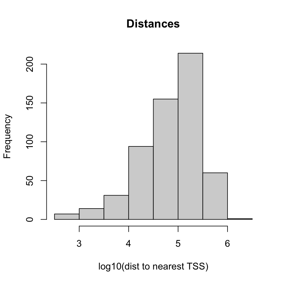
FIGURE 6.2: Histogram of distances of CpG islands to the nearest TSSes.