3.2 How to test for differences between samples

Oftentimes we would want to compare sets of samples. Such comparisons include if wild-type samples have different expression compared to mutants or if healthy samples are different from disease samples in some measurable feature (blood count, gene expression, methylation of certain loci). Since there is variability in our measurements, we need to take that into account when comparing the sets of samples. We can simply subtract the means of two samples, but given the variability of sampling, at the very least we need to decide a cutoff value for differences of means; small differences of means can be explained by random chance due to sampling. That means we need to compare the difference we get to a value that is typical to get if the difference between two group means were only due to sampling. If you followed the logic above, here we actually introduced two core ideas of something called “hypothesis testing”, which is simply using statistics to determine the probability that a given hypothesis (Ex: if two sample sets are from the same population or not) is true. Formally, expanded version of those two core ideas are as follows:

Decide on a hypothesis to test, often called the “null hypothesis” (\(H_0\)). In our case, the hypothesis is that there is no difference between sets of samples. An “alternative hypothesis” (\(H_1\)) is that there is a difference between the samples.
Decide on a statistic to test the truth of the null hypothesis.
Calculate the statistic.
Compare it to a reference value to establish significance, the P-value. Based on that, either reject or not reject the null hypothesis, \(H_0\).

3.2.1 Randomization-based testing for difference of the means

There is one intuitive way to go about this. If we believe there are no differences between samples, that means the sample labels (test vs. control or healthy vs. disease) have no meaning. So, if we randomly assign labels to the samples and calculate the difference of the means, this creates a null distribution for \(H_0\) where we can compare the real difference and measure how unlikely it is to get such a value under the expectation of the null hypothesis. We can calculate all possible permutations to calculate the null distribution. However, sometimes that is not very feasible and the equivalent approach would be generating the null distribution by taking a smaller number of random samples with shuffled group membership.

Below, we are doing this process in R. We are first simulating two samples from two different distributions. These would be equivalent to gene expression measurements obtained under different conditions. Then, we calculate the differences in the means and do the randomization procedure to get a null distribution when we assume there is no difference between samples, \(H_0\). We then calculate how often we would get the original difference we calculated under the assumption that \(H_0\) is true. The resulting null distribution and the original value is shown in Figure 3.9.

set.seed(100)
gene1=rnorm(30,mean=4,sd=2)
gene2=rnorm(30,mean=2,sd=2)
org.diff=mean(gene1)-mean(gene2)
gene.df=data.frame(exp=c(gene1,gene2),
                  group=c( rep("test",30),rep("control",30) ) )


exp.null <- do(1000) * diff(mosaic::mean(exp ~ shuffle(group), data=gene.df))
hist(exp.null[,1],xlab="null distribution | no difference in samples",
     main=expression(paste(H[0]," :no difference in means") ),
     xlim=c(-2,2),col="cornflowerblue",border="white")
abline(v=quantile(exp.null[,1],0.95),col="red" )
abline(v=org.diff,col="blue" )
text(x=quantile(exp.null[,1],0.95),y=200,"0.05",adj=c(1,0),col="red")
text(x=org.diff,y=200,"org. diff.",adj=c(1,0),col="blue")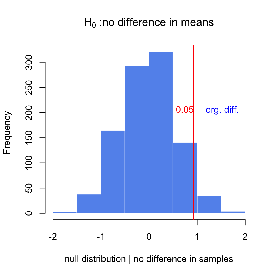

The null distribution for differences of means obtained via randomization. The original difference is marked via the blue line. The red line marks the value that corresponds to P-value of 0.05

FIGURE 3.9: The null distribution for differences of means obtained via randomization. The original difference is marked via the blue line. The red line marks the value that corresponds to P-value of 0.05

p.val=sum(exp.null[,1]>org.diff)/length(exp.null[,1])
p.val

## [1] 0.001

After doing random permutations and getting a null distribution, it is possible to get a confidence interval for the distribution of difference in means. This is simply the \(2.5th\) and \(97.5th\) percentiles of the null distribution, and directly related to the P-value calculation above.

3.2.2 Using t-test for difference of the means between two samples

We can also calculate the difference between means using a t-test. Sometimes we will have too few data points in a sample to do a meaningful randomization test, also randomization takes more time than doing a t-test. This is a test that depends on the t distribution. The line of thought follows from the CLT and we can show differences in means are t distributed. There are a couple of variants of the t-test for this purpose. If we assume the population variances are equal we can use the following version

\[t = \frac{\bar {X}_1 - \bar{X}_2}{s_{X_1X_2} \cdot \sqrt{\frac{1}{n_1}+\frac{1}{n_2}}}\] where \[s_{X_1X_2} = \sqrt{\frac{(n_1-1)s_{X_1}^2+(n_2-1)s_{X_2}^2}{n_1+n_2-2}}\] In the first equation above, the quantity is t distributed with \(n_1+n_2-2\) degrees of freedom. We can calculate the quantity and then use software to look for the percentile of that value in that t distribution, which is our P-value. When we cannot assume equal variances, we use “Welch’s t-test” which is the default t-test in R and also works well when variances and the sample sizes are the same. For this test we calculate the following quantity:

\[t = \frac{\overline{X}_1 - \overline{X}_2}{s_{\overline{X}_1 - \overline{X}_2}}\] where \[s_{\overline{X}_1 - \overline{X}_2} = \sqrt{\frac{s_1^2 }{ n_1} + \frac{s_2^2 }{n_2}}\]

and the degrees of freedom equals to

\[\mathrm{d.f.} = \frac{(s_1^2/n_1 + s_2^2/n_2)^2}{(s_1^2/n_1)^2/(n_1-1) + (s_2^2/n_2)^2/(n_2-1)} \]

Luckily, R does all those calculations for us. Below we will show the use of t.test() function in R. We will use it on the samples we simulated above.

# Welch's t-test
stats::t.test(gene1,gene2)

## 
##  Welch Two Sample t-test
## 
## data:  gene1 and gene2
## t = 3.7653, df = 47.552, p-value = 0.0004575
## alternative hypothesis: true difference in means is not equal to 0
## 95 percent confidence interval:
##  0.872397 2.872761
## sample estimates:
## mean of x mean of y 
##  4.057728  2.185149

# t-test with equal variance assumption
stats::t.test(gene1,gene2,var.equal=TRUE)

## 
##  Two Sample t-test
## 
## data:  gene1 and gene2
## t = 3.7653, df = 58, p-value = 0.0003905
## alternative hypothesis: true difference in means is not equal to 0
## 95 percent confidence interval:
##  0.8770753 2.8680832
## sample estimates:
## mean of x mean of y 
##  4.057728  2.185149

A final word on t-tests: they generally assume a population where samples coming from them have a normal distribution, however it is been shown t-test can tolerate deviations from normality, especially, when two distributions are moderately skewed in the same direction. This is due to the central limit theorem, which says that the means of samples will be distributed normally no matter the population distribution if sample sizes are large.

3.2.3 Multiple testing correction

We should think of hypothesis testing as a non-error-free method of making decisions. There will be times when we declare something significant and accept \(H_1\) but we will be wrong. These decisions are also called “false positives” or “false discoveries”, and are also known as “type I errors”. Similarly, we can fail to reject a hypothesis when we actually should. These cases are known as “false negatives”, also known as “type II errors”.

The ratio of true negatives to the sum of true negatives and false positives (\(\frac{TN}{FP+TN}\)) is known as specificity. And we usually want to decrease the FP and get higher specificity. The ratio of true positives to the sum of true positives and false negatives (\(\frac{TP}{TP+FN}\)) is known as sensitivity. And, again, we usually want to decrease the FN and get higher sensitivity. Sensitivity is also known as the “power of a test” in the context of hypothesis testing. More powerful tests will be highly sensitive and will have fewer type II errors. For the t-test, the power is positively associated with sample size and the effect size. The larger the sample size, the smaller the standard error, and looking for the larger effect sizes will similarly increase the power.

The general summary of these different decision combinations are included in the table below.

	\(H_0\) is TRUE, [Gene is NOT differentially expressed]	\(H_1\) is TRUE, [Gene is differentially expressed]
Accept \(H_0\) (claim that the gene is not differentially expressed)	True Negatives (TN)	False Negatives (FN) ,type II error	\(m_0\): number of truly null hypotheses
reject \(H_0\) (claim that the gene is differentially expressed)	False Positives (FP) ,type I error	True Positives (TP)	\(m-m_0\): number of truly alternative hypotheses

We expect to make more type I errors as the number of tests increase, which means we will reject the null hypothesis by mistake. For example, if we perform a test at the 5% significance level, there is a 5% chance of incorrectly rejecting the null hypothesis if the null hypothesis is true. However, if we make 1000 tests where all null hypotheses are true for each of them, the average number of incorrect rejections is 50. And if we apply the rules of probability, there is almost a 100% chance that we will have at least one incorrect rejection. There are multiple statistical techniques to prevent this from happening. These techniques generally push the P-values obtained from multiple tests to higher values; if the individual P-value is low enough it survives this process. The simplest method is just to multiply the individual P-value (\(p_i\)) by the number of tests (\(m\)), \(m \cdot p_i\). This is called “Bonferroni correction”. However, this is too harsh if you have thousands of tests. Other methods are developed to remedy this. Those methods rely on ranking the P-values and dividing \(m \cdot p_i\) by the rank, \(i\), :\(\frac{m \cdot p_i }{i}\), which is derived from the Benjamini–Hochberg procedure. This procedure is developed to control for “False Discovery Rate (FDR)” , which is the proportion of false positives among all significant tests. And in practical terms, we get the “FDR-adjusted P-value” from the procedure described above. This gives us an estimate of the proportion of false discoveries for a given test. To elaborate, p-value of 0.05 implies that 5% of all tests will be false positives. An FDR-adjusted p-value of 0.05 implies that 5% of significant tests will be false positives. The FDR-adjusted P-values will result in a lower number of false positives.

One final method that is also popular is called the “q-value” method and related to the method above. This procedure relies on estimating the proportion of true null hypotheses from the distribution of raw p-values and using that quantity to come up with what is called a “q-value”, which is also an FDR-adjusted P-value (Storey and Tibshirani 2003). That can be practically defined as “the proportion of significant features that turn out to be false leads.” A q-value 0.01 would mean 1% of the tests called significant at this level will be truly null on average. Within the genomics community q-value and FDR adjusted P-value are synonymous although they can be calculated differently.

In R, the base function p.adjust() implements most of the p-value correction methods described above. For the q-value, we can use the qvalue package from Bioconductor. Below we demonstrate how to use them on a set of simulated p-values. The plot in Figure 3.10 shows that Bonferroni correction does a terrible job. FDR(BH) and q-value approach are better but, the q-value approach is more permissive than FDR(BH).

library(qvalue)
data(hedenfalk)

qvalues <- qvalue(hedenfalk$p)$q
bonf.pval=p.adjust(hedenfalk$p,method ="bonferroni")
fdr.adj.pval=p.adjust(hedenfalk$p,method ="fdr")

plot(hedenfalk$p,qvalues,pch=19,ylim=c(0,1),
     xlab="raw P-values",ylab="adjusted P-values")
points(hedenfalk$p,bonf.pval,pch=19,col="red")
points(hedenfalk$p,fdr.adj.pval,pch=19,col="blue")
legend("bottomright",legend=c("q-value","FDR (BH)","Bonferroni"),
       fill=c("black","blue","red"))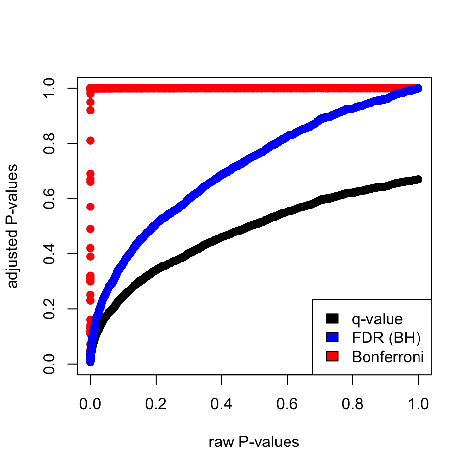

FIGURE 3.10: Adjusted P-values via different methods and their relationship to raw P-values

3.2.4 Moderated t-tests: Using information from multiple comparisons

In genomics, we usually do not do one test but many, as described above. That means we may be able to use the information from the parameters obtained from all comparisons to influence the individual parameters. For example, if you have many variances calculated for thousands of genes across samples, you can force individual variance estimates to shrink toward the mean or the median of the distribution of variances. This usually creates better performance in individual variance estimates and therefore better performance in significance testing, which depends on variance estimates. How much the values are shrunk toward a common value depends on the exact method used. These tests in general are called moderated t-tests or shrinkage t-tests. One approach popularized by Limma software is to use so-called “Empirical Bayes methods”. The main formulation in these methods is \(\hat{V_g} = aV_0 + bV_g\), where \(V_0\) is the background variability and \(V_g\) is the individual variability. Then, these methods estimate \(a\) and \(b\) in various ways to come up with a “shrunk” version of the variability, \(\hat{V_g}\). Bayesian inference can make use of prior knowledge to make inference about properties of the data. In a Bayesian viewpoint, the prior knowledge, in this case variability of other genes, can be used to calculate the variability of an individual gene. In our case, \(V_0\) would be the prior knowledge we have on the variability of the genes and we use that knowledge to influence our estimate for the individual genes.

Below we are simulating a gene expression matrix with 1000 genes, and 3 test and 3 control groups. Each row is a gene, and in normal circumstances we would like to find differentially expressed genes. In this case, we are simulating them from the same distribution, so in reality we do not expect any differences. We then use the adjusted standard error estimates in empirical Bayesian spirit but, in a very crude way. We just shrink the gene-wise standard error estimates towards the median with equal \(a\) and \(b\) weights. That is to say, we add the individual estimate to the median of the standard error distribution from all genes and divide that quantity by 2. So if we plug that into the above formula, what we do is:

\[ \hat{V_g} = (V_0 + V_g)/2 \]

In the code below, we are avoiding for loops or apply family functions by using vectorized operations. The code below samples gene expression values from a hypothetical distribution. Since all the values come from the same distribution, we do not expect differences between groups. We then calculate moderated and unmoderated t-test statistics and plot the P-value distributions for tests. The results are shown in Figure 3.11.

set.seed(100)

#sample data matrix from normal distribution

gset=rnorm(3000,mean=200,sd=70)
data=matrix(gset,ncol=6)

# set groups
group1=1:3
group2=4:6
n1=3
n2=3
dx=rowMeans(data[,group1])-rowMeans(data[,group2])
  
require(matrixStats)

# get the esimate of pooled variance 
stderr = sqrt( (rowVars(data[,group1])*(n1-1) + 
       rowVars(data[,group2])*(n2-1)) / (n1+n2-2) * ( 1/n1 + 1/n2 ))

# do the shrinking towards median
mod.stderr = (stderr + median(stderr)) / 2 # moderation in variation

# esimate t statistic with moderated variance
t.mod <- dx / mod.stderr

# calculate P-value of rejecting null 
p.mod = 2*pt( -abs(t.mod), n1+n2-2 )

# esimate t statistic without moderated variance
t = dx / stderr

# calculate P-value of rejecting null 
p = 2*pt( -abs(t), n1+n2-2 )

par(mfrow=c(1,2))
hist(p,col="cornflowerblue",border="white",main="",xlab="P-values t-test")
mtext(paste("signifcant tests:",sum(p<0.05))  )
hist(p.mod,col="cornflowerblue",border="white",main="",
     xlab="P-values mod. t-test")
mtext(paste("signifcant tests:",sum(p.mod<0.05))  )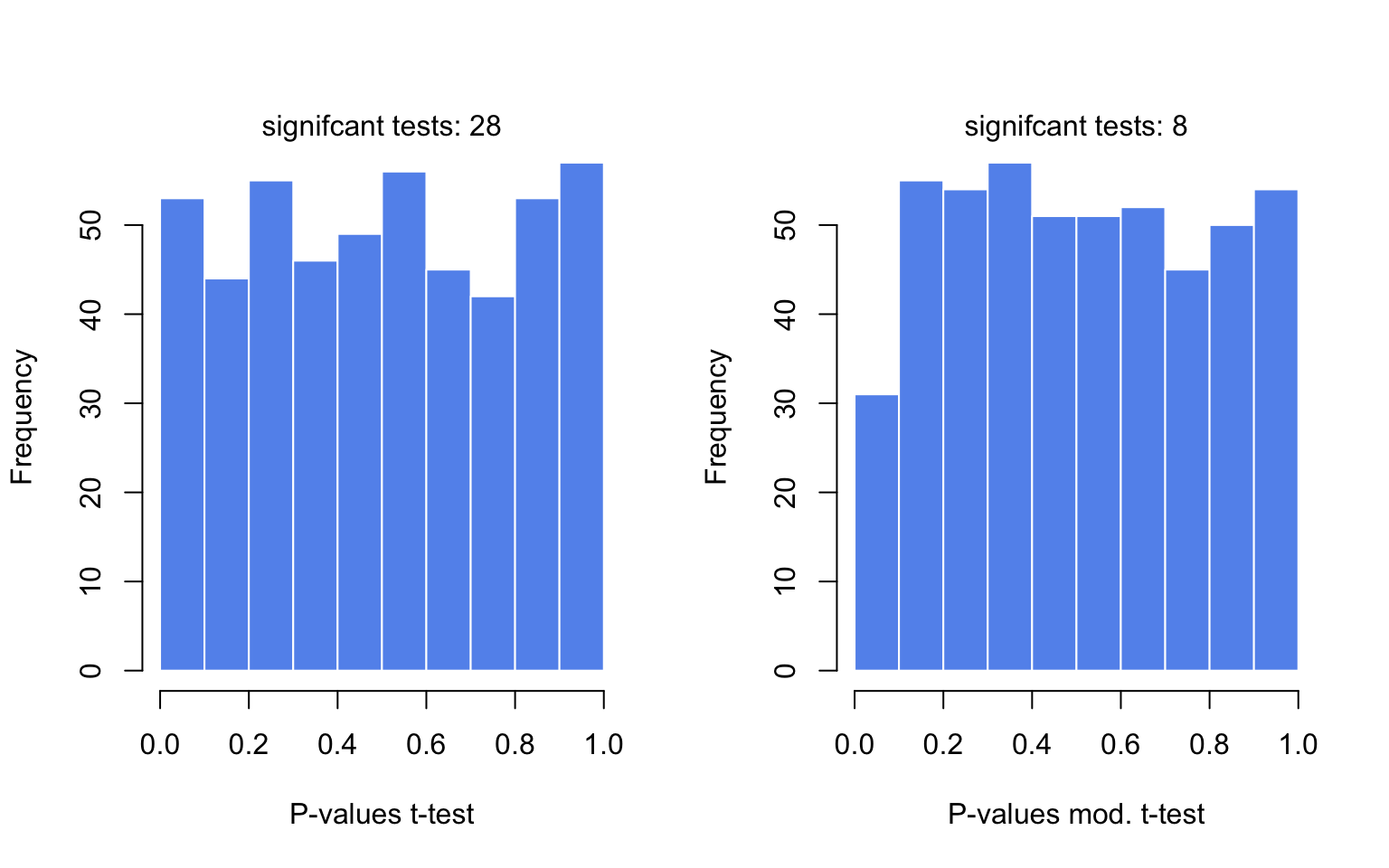

FIGURE 3.11: The distributions of P-values obtained by t-tests and moderated t-tests

Want to know more ?

Basic statistical concepts
- “Cartoon guide to statistics” by Gonick & Smith (Gonick and Smith 2005). Provides central concepts depicted as cartoons in a funny but clear and accurate manner.
- “OpenIntro Statistics” (Diez, Barr, Çetinkaya-Rundel, et al. 2015) (Free e-book http://openintro.org). This book provides fundamental statistical concepts in a clear and easy way. It includes R code.
Hands-on statistics recipes with R
- “The R book” (Crawley 2012). This is the main R book for anyone interested in statistical concepts and their application in R. It requires some background in statistics since the main focus is applications in R.
Moderated tests
- Comparison of moderated tests for differential expression (De Hertogh, De Meulder, Berger, et al. 2010) http://bmcbioinformatics.biomedcentral.com/articles/10.1186/1471-2105-11-17
- Limma method developed for testing differential expression between genes using a moderated test (Smyth Gordon 2004) http://www.statsci.org/smyth/pubs/ebayes.pdf

References

Crawley. 2012. The R Book. Wiley. https://books.google.de/books?id=XYDl0mlH-moC.

De Hertogh, De Meulder, Berger, Pierre, Bareke, Gaigneaux, and Depiereux. 2010. “A Benchmark for Statistical Microarray Data Analysis That Preserves Actual Biological and Technical Variance.” BMC Bioinformatics 11 (1): 17.

Diez, Barr, Çetinkaya-Rundel, and Amazon.com. 2015. OpenIntro Statistics. OpenIntro, Incorporated. https://books.google.de/books?id=wfcPswEACAAJ.

Gonick, and Smith. 2005. The Cartoon Guide to Statistics. Collins Reference. https://books.google.de/books?id=-U7vygAACAAJ.

Smyth Gordon. 2004. “Linear Models and Empirical Bayes Methods for Assessing Differential Expression in Microarray Experiments.” Statistical Applications in Genetics and Molecular Biology 3 (1): 1–25.

Storey, and Tibshirani. 2003. “Statistical Significance for Genomewide Studies.” Proc. Natl. Acad. Sci. U. S. A. 100 (16): 9440–5.