3.4 Exercises
3.4.1 How to summarize collection of data points: The idea behind statistical distributions
- Calculate the means and variances
of the rows of the following simulated data set, and plot the distributions
of means and variances using
hist()andboxplot()functions. [Difficulty: Beginner/Intermediate]
set.seed(100)

#sample data matrix from normal distribution
gset=rnorm(600,mean=200,sd=70)
data=matrix(gset,ncol=6)
Using the data generated above, calculate the standard deviation of the distribution of the means using the
sd()function. Compare that to the expected standard error obtained from the central limit theorem keeping in mind the population parameters were \(\sigma=70\) and \(n=6\). How does the estimate from the random samples change if we simulate more data withdata=matrix(rnorm(6000,mean=200,sd=70),ncol=6)? [Difficulty: Beginner/Intermediate]Simulate 30 random variables using the
rpois()function. Do this 1000 times and calculate the mean of each sample. Plot the sampling distributions of the means using a histogram. Get the 2.5th and 97.5th percentiles of the distribution. [Difficulty: Beginner/Intermediate]Use the
t.test()function to calculate confidence intervals of the mean on the first random samplepois1simulated from therpois()function below. [Difficulty: Intermediate]
#HINT
set.seed(100)

#sample 30 values from poisson dist with lamda paramater =30
pois1=rpois(30,lambda=5)- Use the bootstrap confidence interval for the mean on
pois1. [Difficulty: Intermediate/Advanced] - Compare the theoretical confidence interval of the mean from the
t.testand the bootstrap confidence interval. Are they similar? [Difficulty: Intermediate/Advanced]
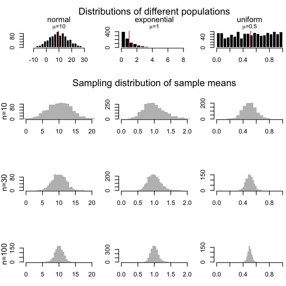
- Try to re-create the following figure, which demonstrates the CLT concept.[Difficulty: Advanced]
3.4.2 How to test for differences in samples
- Test the difference of means of the following simulated genes
using the randomization,
t-test(), andwilcox.test()functions. Plot the distributions using histograms and boxplots. [Difficulty: Intermediate/Advanced]
- Test the difference of the means of the following simulated genes
using the randomization,
t-test()andwilcox.test()functions. Plot the distributions using histograms and boxplots. [Difficulty: Intermediate/Advanced]
- We need an extra data set for this exercise. Read the gene expression data set as follows:
gexpFile=system.file("extdata","geneExpMat.rds",package="compGenomRData") data=readRDS(gexpFile). The data has 100 differentially expressed genes. The first 3 columns are the test samples, and the last 3 are the control samples. Do a t-test for each gene (each row is a gene), and record the p-values. Then, do a moderated t-test, as shown in section “Moderated t-tests” in this chapter, and record the p-values. Make a p-value histogram and compare two approaches in terms of the number of significant tests with the \(0.05\) threshold. On the p-values use FDR (BH), Bonferroni and q-value adjustment methods. Calculate how many adjusted p-values are below 0.05 for each approach. [Difficulty: Intermediate/Advanced]
3.4.3 Relationship between variables: Linear models and correlation
Below we are going to simulate X and Y values that are needed for the rest of the exercise.
# set random number seed, so that the random numbers from the text
# is the same when you run the code.
set.seed(32)

# get 50 X values between 1 and 100
x = runif(50,1,100)

# set b0,b1 and variance (sigma)
b0 = 10
b1 = 2
sigma = 20
# simulate error terms from normal distribution
eps = rnorm(50,0,sigma)
# get y values from the linear equation and addition of error terms
y = b0 + b1*x+ eps
Run the code then fit a line to predict Y based on X. [Difficulty:Intermediate]
Plot the scatter plot and the fitted line. [Difficulty:Intermediate]
Calculate correlation and R^2. [Difficulty:Intermediate]
Run the
summary()function and try to extract P-values for the model from the object returned bysummary. See?summary.lm. [Difficulty:Intermediate/Advanced]Plot the residuals vs. the fitted values plot, by calling the
plot()function withwhich=1as the second argument. First argument is the model returned bylm(). [Difficulty:Advanced]For the next exercises, read the data set histone modification data set. Use the following to get the path to the file:
hmodFile=system.file("extdata",
                    "HistoneModeVSgeneExp.rds",
                     package="compGenomRData")`
There are 3 columns in the dataset. These are measured levels of H3K4me3, H3K27me3 and gene expression per gene. Once you read in the data, plot the scatter plot for H3K4me3 vs. expression. [Difficulty:Beginner]
Plot the scatter plot for H3K27me3 vs. expression. [Difficulty:Beginner]
Fit the model for prediction of expression data using: 1) Only H3K4me3 as explanatory variable, 2) Only H3K27me3 as explanatory variable, and 3) Using both H3K4me3 and H3K27me3 as explanatory variables. Inspect the
summary()function output in each case, which terms are significant. [Difficulty:Beginner/Intermediate]Is using H3K4me3 and H3K27me3 better than the model with only H3K4me3? [Difficulty:Intermediate]
Plot H3k4me3 vs. H3k27me3. Inspect the points that do not follow a linear trend. Are they clustered at certain segments of the plot? Bonus: Is there any biological or technical interpretation for those points? [Difficulty:Intermediate/Advanced]