9.6 Peak calling
After we are convinced that the data is of sufficient quality, we can proceed with the downstream analysis. One of the first steps in the ChIP-seq analysis is peak calling. Peak calling is a statistical procedure, which uses coverage properties of ChIP and Input samples to find regions which are enriched due to protein binding. The procedure requires mapped reads, and outputs a set of regions, which represent the putative binding locations. Each region is usually associated with a significance score which is an indicator of enrichment.
For peak calling we will use the normR Bioconductor package.
normR uses a binomial mixture model, and performs simultaneous
normalization and peak finding. Due to the nature of the model, it is
quite flexible and can be used for different types of ChIP experiments.
One of the caveats of normR is that it does not inherently support
multiple biological replicates, for the same biological sample.
Therefore, the peak calling procedure needs to be done on each replicate
separately, and the peaks need to be combined in post-processing.
9.6.1 Types of ChIP-seq experiments
Based on the binding properties of ChIP-ped proteins, ChIP-seq signal profiles can be divided into three classes:
Sharp (point signal): A signal profile which is localized to specific short genomic regions (up to couple of hundred base pairs) It is usually obtained from transcription factors, or highly localized posttranslational histone modifications (H3K4me3, which is found on gene promoters).
Broad (wide signal): The signal covers broad genomic domains spanning up to several kilobases. Usually produced by disperse histone modifications (H3K36me3, located on gene bodies, or H3K23me3, which is deposited by the Polycomb complex in large genomic regions).
Mixed: The signal consists of a mixture of sharp and broad regions. It is produced by proteins which have dynamic behavior. Most often these are ChIP experiments of RNA Polymerase 2.
Different types of ChIP experiments usually require specialized analysis tools. Some peak callers are developed to specifically detect narrow peaks (Zhang, Liu, Meyer, et al. 2008; Xu, Handoko, Wei, et al. 2010; Shao, Zhang, Yuan, et al. 2012), while others
detect enrichment in diffuse broad regions (Zang, Schones, Zeng, et al. 2009; Micsinai, Parisi, Strino, et al. 2012; Beck, Brandl, Boelen, et al. 2012; Song and Smith 2011; Xing, Mo, Liao, et al. 2012),
or mixed (Polymerase 2) signals (Han, Tian, Pécot, et al. 2012).
Recent developments in peak calling methods (such as normR) can however accommodate
multiple types of ChIP experiments (Rashid, Giresi, Ibrahim, et al. 2011).
The choice of the algorithm will largely depend on the type of the wanted
results, and the peculiarities of the experimental design and execution (Laajala, Raghav, Tuomela, et al. 2009; Wilbanks and Facciotti 2010).
If you are not certain what kind of signal profile to expect from a ChIP-seq experiment, the best solution is to visualize the data. We will now use the data from H3K4me3 (Sharp), H3K36me3 (Broad), and POL2 (Mixed) ChIP experiments to show the differences in the signal profiles. We will use the bigWig files to visualize the signal profiles around a highly expressed human gene from chromosome 21. This will give us an indication of how the profiles for different types of ChIP experiments differ. First we select the files of interest:
# set names for chip-seq bigWig files
chip_files = list(
    H3K4me3  = 'GM12878_hg38_H3K4me3.chr21.bw',

    H3K36me3 = 'GM12878_hg38_H3K36me3.chr21.bw',

    POL2     = 'GM12878_hg38_POLR2A.chr21.bw'
)
# get full paths to the files
chip_files = lapply(chip_files, function(x){
    file.path(data_path, x)
})
Next we import the coverage profiles into R:
# load rtracklayer
library(rtracklayer)

# import the ChIP bigWig files
chip_profiles = lapply(chip_files, rtracklayer::import.bw)
We fetch the reference annotation for human chromosome 21.
library(AnnotationHub)
hub = AnnotationHub()
gtf = hub[['AH61126']]

# select only chromosome 21
seqlevels(gtf, pruning.mode='coarse') = '21'

# extract chromosome names
ensembl_seqlevels = seqlevels(gtf)

# paste the chr prefix to the chromosome names
ucsc_seqlevels    = paste0('chr', ensembl_seqlevels)

# replace ensembl with ucsc chromosome names
seqlevels(gtf, pruning.mode='coarse') = ucsc_seqlevels
To enable Gviz to work with genomic annotation we will convert the GRanges
object into a transcript database using the following function:
# load the GenomicFeatures object
library(GenomicFeatures)

# convert the gtf annotation into a data.base
txdb         = makeTxDbFromGRanges(gtf)
And convert the transcript database into a Gviz track.
Once we have downloaded the annotation, and imported the signal profiles into R we are ready to visualize the data.
We will again use the Gviz library. We firstly define the coordinate system. The ideogram track which will show
the position of our current viewpoint on the chromosome, and a genome axis track, which will show the exact coordinates.
# load Gviz package
library(Gviz)
# fetches the chromosome length information
hg_chrs = getChromInfoFromUCSC('hg38')
hg_chrs = subset(hg_chrs, (grepl('chr21$',chrom)))

# convert data.frame to named vector
seqlengths = with(hg_chrs, setNames(size, chrom))

# constructs the ideogram track
chr_track   = IdeogramTrack(
    chromosome = 'chr21',
    genome     = 'hg38'
)

# constructs the coordinate system
axis = GenomeAxisTrack(
    range = GRanges('chr21', IRanges(1, width=seqlengths))
)
We use a loop to convert the signal profiles into a DataTrack object.
# use a lapply on the imported bw files to create the track objects
# we loop over experiment names, and select the corresponding object
# within the function
data_tracks = lapply(names(chip_profiles), function(exp_name){

    # chip_profiles[[exp_name]] - selects the
    # proper experiment using the exp_name
    DataTrack(
        range = chip_profiles[[exp_name]],
        name  = exp_name,

        # type of the track
        type  = 'h',

        # line width parameter
        lwd   = 5
    )
})
We are finally ready to create the genome screenshot. We will focus on an extended region around the URB1 gene.
# select the start coordinate for the URB1 gene
start = min(start(subset(gtf, gene_name == 'URB1')))

# select the end coordinate for the URB1 gene
end   = max(end(subset(gtf, gene_name == 'URB1')))

# plot the signal profiles around the URB1 gene
plotTracks(
    trackList = c(chr_track, axis, gene_track, data_tracks),

    # relative track sizes
    sizes     = c(1,1,1,1,1,1),

    # background color
    background.title     = "black",

    # controls visualization of gene sets
    collapseTranscripts  = "longest",
    transcriptAnnotation = "symbol",

    # coordinates to visualize
    from = start - 5000,
    to   = end   + 5000
)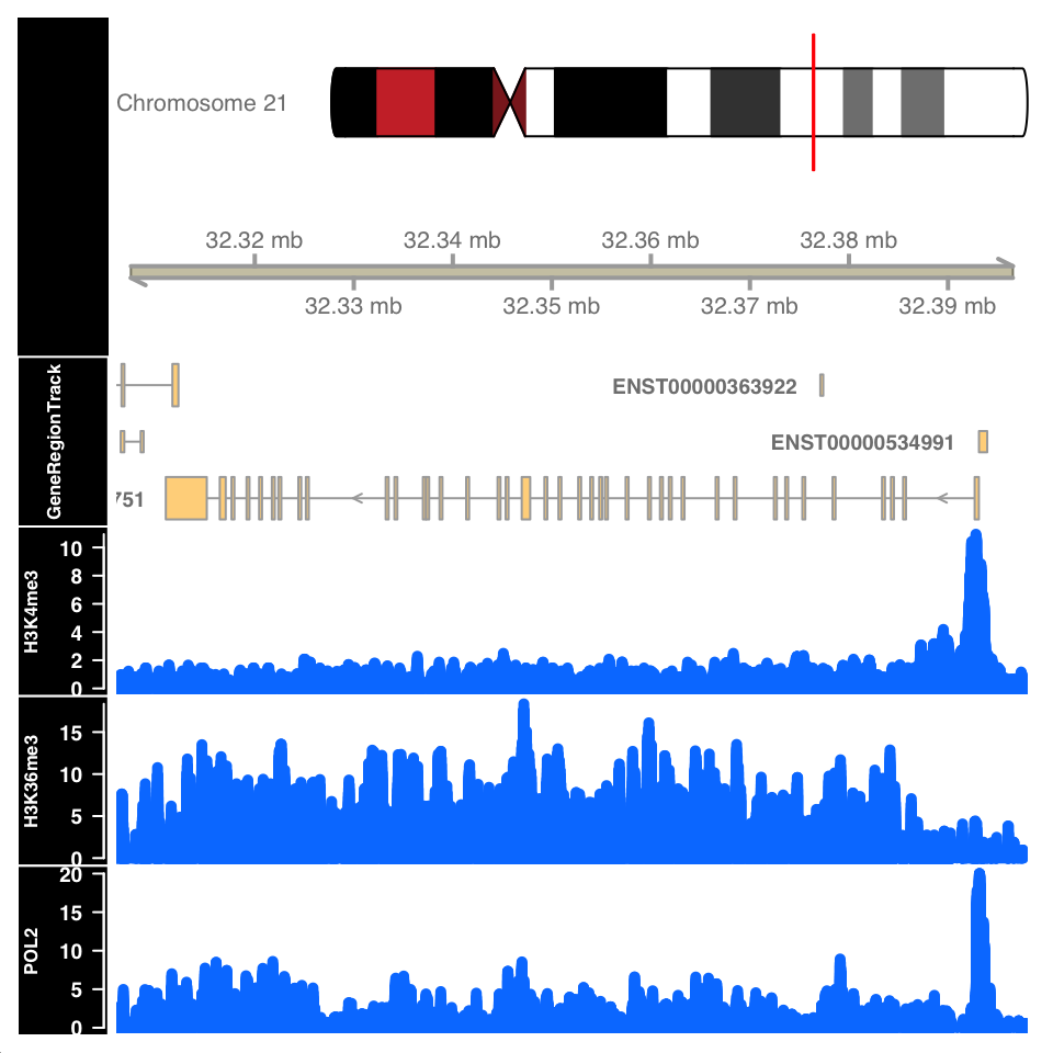
FIGURE 9.11: ChIP-seq signal around the URB1 gene.
Figure 9.11 shows the signal profile around the URB1 gene. H3K4me3 signal profile contains a strong narrow peak on the transcription start site. H3K36me3 shows strong enrichment in the gene body, while the POL2 ChIP shows a mixed profile, with a strong peak at the TSS and an enrichment over the gene body.
9.6.2 Peak calling: Sharp peaks
We will now use the normR (Helmuth, Li, Arrigoni, et al. 2016) package for peak calling in sharp and broad peak experiments.
Select the input files. Since normR does not support the usage of biological
replicates, we will showcase the peak calling on one of the CTCF samples.
# full path to the ChIP data file
chip_file    = file.path(data_path, 'GM12878_hg38_CTCF_r1.chr21.bam')

# full path to the Control data file
control_file = file.path(data_path, 'GM12878_hg38_Input_r5.chr21.bam')
To understand the dynamic range of enrichment, we will create a scatter plot showing the strength of signal in the CTCF and Input.
Let us first count the reads in 1-kb windows, and normalize them to counts per million sequenced reads.
# as previously done, we calculate the cpm for each experiment
library(GenomicRanges)
library(GenomicAlignments)

# select the chromosome
hg_chrs = getChromInfoFromUCSC('hg38')
hg_chrs = subset(hg_chrs, grepl('chr21$',chrom))

seqlengths = with(hg_chrs, setNames(size, chrom))

# define the windows
tilling_window = unlist(tileGenome(seqlengths, tilewidth=1000))

# count the reads
counts         = summarizeOverlaps(
    features = tilling_window,
    reads    = c(chip_file, control_file)
)

# normalize read counts
counts         = assays(counts)[[1]]
cpm = t(t(counts)*(1000000/colSums(counts)))
We can now plot the ChIP versus Input signal:
library(ggplot2)
# convert the matrix into a data.frame for ggplot
cpm = data.frame(cpm)
ggplot(
    data = cpm,
    aes(
        x = GM12878_hg38_Input_r5.chr21.bam,
        y = GM12878_hg38_CTCF_r1.chr21.bam)
    ) +
    geom_point() +
    geom_abline(slope = 1) +
    theme_bw() +
    theme_bw() +
    scale_fill_brewer(palette='Set2') +
    theme(
        axis.text   = element_text(size=10, face='bold'),
        axis.title  = element_text(size=14,face="bold"),
        plot.title  = element_text(hjust = 0.5),
        axis.text.x = element_text(angle = 90, hjust = 1)) +
    xlab('Input CPM') +
    ylab('CTCF CPM') +
    ggtitle('ChIP versus Input')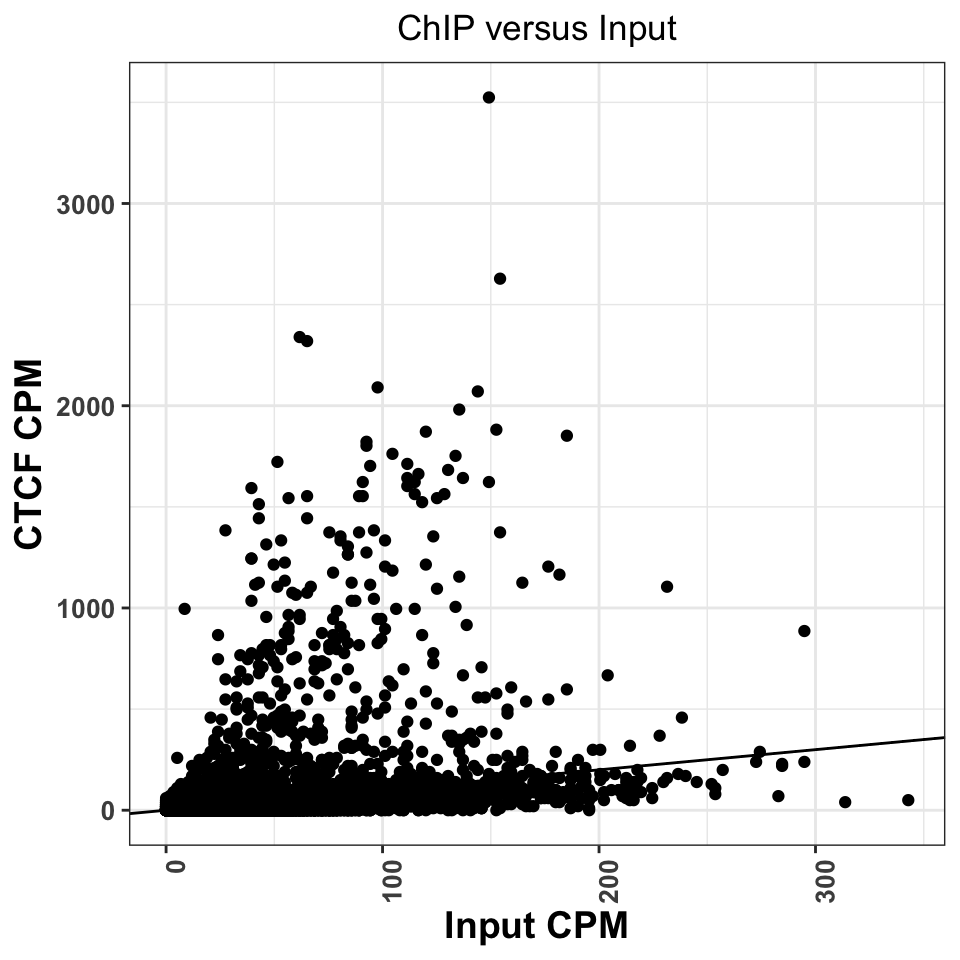
FIGURE 9.12: Comparison of CPM values between ChIP and Input experiments. Good ChIP experiments should always show enrichment.
Regions above the diagonal, in Figure 9.12, show higher enrichment in the ChIP samples, while the regions below the diagonal show higher enrichment in the Input samples.
Let us now perform for peak calling. normR usage is deceivingly simple; we need to provide the location ChIP and Control read files, and the genome version to the enrichR() function. The function will automatically create tilling windows (250bp by default), count the number of reads in each window, and fit a mixture of binomial distributions.
library(normr)
# peak calling using chip and control
ctcf_fit = enrichR(

            # ChIP file
            treatment = chip_file,

            # control file
            control   = control_file,

            # genome version
            genome    = "hg38",

            # print intermediary steps during the analysis
            verbose   = FALSE)
With the summary function we can take a look at the results:
## NormRFit-class object
##
## Type:                  'enrichR'
## Number of Regions:     12353090
## Number of Components:  2
## Theta* (naive bg):     0.137
## Background component B: 1
##
## +++ Results of fit +++
## Mixture Proportions:
## Background       Class 1
##     97.72%         2.28%
## Theta:
## Background       Class 1
##      0.103         0.695
##
## Bayesian Information Criterion:  539882
##
## +++ Results of binomial test +++
## T-Filter threshold: 4
## Number of Regions filtered out: 12267164
## Significantly different from background B based on q-values:
## TOTAL:
##            ***        **         *         .                n.s.
## Bins         0       627       120       195        87     84897
## %        0.000     0.711     0.847     1.068     1.166    96.209
## ---
## Signif. codes:  0 '***' 0.001 '**' 0.01 '*' 0.05 '.' 0.1 '  ' 1 'n.s.'
The summary function shows that most of the regions of chromosome 21 correspond to the background: \(97.72%\). In total we have \(1029=(627+120+195+87)\) significantly enriched regions.
We will now extract the regions into a GRanges object.
The getRanges() function extracts the regions from the model. Using the
getQvalue(), and getEnrichment() function we assign to our regions
the statistical significance and calculated enrichment.
In order to identify only highly significant regions,
we keep only ranges where the false discovery rate (q value) is below \(0.01\).
# extracts the ranges
ctcf_peaks = getRanges(ctcf_fit)

# annotates the ranges with the supporting p value
ctcf_peaks$qvalue     = getQvalues(ctcf_fit)

# annotates the ranges with the calculated enrichment
ctcf_peaks$enrichment = getEnrichment(ctcf_fit)

# selects the ranges which correspond to the enriched class
ctcf_peaks = subset(ctcf_peaks, !is.na(component))

# filter by a stringent q value threshold
ctcf_peaks = subset(ctcf_peaks, qvalue < 0.01)

# order the peaks based on the q value
ctcf_peaks = ctcf_peaks[order(ctcf_peaks$qvalue)]
## GRanges object with 724 ranges and 3 metadata columns:
## seqnames ranges strand | component qvalue enrichment
## <Rle> <IRanges> <Rle> | <integer> <numeric> <numeric>
## [1] chr21 43939251-43939500 * | 1 4.69881e-140 1.37891
## [2] chr21 43646751-43647000 * | 1 2.52006e-137 1.42361
## [3] chr21 43810751-43811000 * | 1 1.86404e-121 1.30519
## [4] chr21 43939001-43939250 * | 1 2.10822e-121 1.19820
## [5] chr21 37712251-37712500 * | 1 6.35711e-118 1.70989
## ... ... ... ... . ... ... ...
## [720] chr21 38172001-38172250 * | 1 0.00867374 0.951189
## [721] chr21 38806001-38806250 * | 1 0.00867374 0.951189
## [722] chr21 42009501-42009750 * | 1 0.00867374 0.656253
## [723] chr21 46153001-46153250 * | 1 0.00867374 0.951189
## [724] chr21 46294751-46295000 * | 1 0.00867374 0.722822
## -------
## seqinfo: 24 sequences from an unspecified genomeAfter stringent q value filtering we are left with \(724\) peaks. For the ease of downstream analysis, we will limit the sequence levels to chromosome 21.
Let’s export the peaks into a .txt file which we can use the downstream in the analysis.
# write the peaks loacations into a txt table
write.table(ctcf_peaks, file.path(data_path, 'CTCF_peaks.txt'),
            row.names=F, col.names=T, quote=F, sep='\t')
We can now repeat the CTCF versus Input plot, and label significantly marked peaks. Using the count overlaps we mark which of our 1-kb regions contained significant peaks.
library(ggplot2)
cpm$enriched_regions = enriched_regions

ggplot(
    data = cpm,
    aes(
        x = GM12878_hg38_Input_r5.chr21.bam,
        y = GM12878_hg38_CTCF_r1.chr21.bam,
        color = enriched_regions
    )) +
  geom_point() +
  geom_abline(slope = 1) +
  theme_bw() +
  scale_fill_brewer(palette='Set2') +
  theme(
    axis.text   = element_text(size=10, face='bold'),
    axis.title  = element_text(size=14,face="bold"),
    plot.title  = element_text(hjust = 0.5),
    axis.text.x = element_text(angle = 90, hjust = 1)) +
  xlab('Input CPM') +
  ylab('CTCF CPM') +
  ggtitle('ChIP versus Input') +
  scale_color_manual(values=c('gray','red'))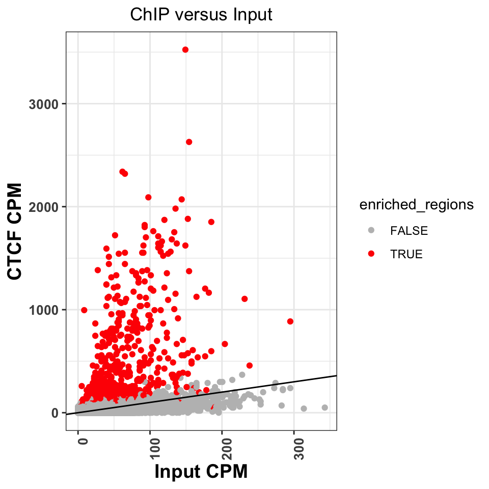
FIGURE 9.13: Comparison of signal between ChIP and input samples. Red labeled dots correspond to called peaks.
Figure 9.13 shows that normR
identified all of the regions above the diagonal as statistically significant.
It has, however, labeled a significant number of regions below the diagonal.
Because of the sophisticated statistical model,
normR has greater sensitivity, and these peaks might really be enriched regions,
it is worth investigating the nature of these regions. This is left as an exercise
to the reader.
We can now create a genome browser screenshot around a peak region. This will show us what kind of signal properties have contributed to the peak calling. We would expect to see a strong, bell-shaped, enrichment in the ChIP sample, and uniform noise in the Input sample.
Let us now visualize the signal around the most enriched peak. The following function takes as input a .bam file, and loads the bam into R. It extends the reads to a size of 200 bp, and creates the coverage vector.
# calculate the coverage for one bam file
calculateCoverage = function(
  bam_file,
  extend = 200
){

  # load reads into R
  reads = readGAlignments(bam_file)

  # convert reads into a GRanges object
  reads = granges(reads)

  # resize the reads to 200bp
  reads = resize(reads, width=extend, fix='start')

  # get the coverage vector
  cov   = coverage(reads)

  # normalize the coverage vector to the sequencing depth
  cov = round(cov * (1000000/length(reads)),2)

  # convert the coverage go a GRanges object
  cov   = as(cov, 'GRanges')

  # keep only chromosome 21
  seqlevels(cov, pruning.mode='coarse') = 'chr21'
  return(cov)
}
Let’s apply the function to the ChIP and input samples.
# calculate coverage for the ChIP file
ctcf_cov = calculateCoverage(chip_file)

# calculate coverage for the control file
cont_cov = calculateCoverage(control_file)
Using Gviz, we will construct the layered tracks.
First, we layout the genome coordinates:
# load Gviz and get the chromosome coordinates
library(Gviz)
chr_track  = IdeogramTrack('chr21', 'hg38')
axis       = GenomeAxisTrack(
    range = GRanges('chr21', IRanges(1, width=seqlengths))
)
Then, the peak locations:
And finally, the signal files:
chip_track  = DataTrack(
    range = ctcf_cov,
    name  = "CTCF",
    type  = 'h',
    lwd   = 3
)

cont_track  = DataTrack(
    range = cont_cov,
    name  = "Input",
    type  = 'h',
    lwd=3
)plotTracks(
trackList = list(chr_track, axis, peaks_track, chip_track, cont_track),
sizes = c(.2,.5,.5,1,1),
background.title = "black",
from = start(ctcf_peaks)[1] - 1000,
to = end(ctcf_peaks)[1] + 1000
)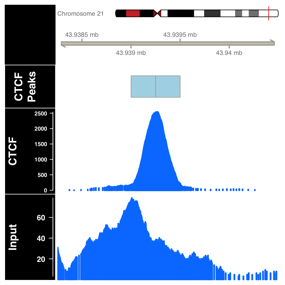
FIGURE 9.14: ChIP and Input signal profile around the peak centers.
In Figure 9.14, the ChIP sample looks as expected. Although the Input sample shows an enrichment, it is important to compare the scales on both samples. The normalized ChIP signal goes up to \(2500\), while the maximum value in the input sample is only \(60\).
9.6.3 Peak calling: Broad regions
We will now use normR to call peaks for the H3K36me3 histone modification,
which is associated with gene bodies of expressed genes. We define the ChIP and Input files:
# fetch the ChIP-file for H3K36me3
chip_file    = file.path(data_path, 'GM12878_hg38_H3K36me3.chr21.bam')

# fetch the corresponding input file
control_file = file.path(data_path, 'GM12878_hg38_Input_r5.chr21.bam')
Because H3K36 regions span broad domains, it is necessary to increase the
tilling window size which will be used for counting.
Using the countConfiguration() function, we will set the tilling window size
to 5000 base pairs.
library(normr)
# define the window width for the counting
countConfiguration = countConfigSingleEnd(binsize = 5000)
# find broad peaks using enrichR
h3k36_fit = enrichR(
# ChIP file
treatment = chip_file,
# control file
control = control_file,
# genome version
genome = "hg38",
verbose = FALSE,
# window size for counting
countConfig = countConfiguration)## NormRFit-class object
##
## Type: 'enrichR'
## Number of Regions: 617665
## Number of Components: 2
## Theta* (naive bg): 0.197
## Background component B: 1
##
## +++ Results of fit +++
## Mixture Proportions:
## Background Class 1
## 85.4% 14.6%
## Theta:
## Background Class 1
## 0.138 0.442
##
## Bayesian Information Criterion: 741525
##
## +++ Results of binomial test +++
## T-Filter threshold: 5
## Number of Regions filtered out: 610736
## Significantly different from background B based on q-values:
## TOTAL:
## *** ** * . n.s.
## Bins 0 1005 314 381 237 4992
## % 0.00 9.18 12.04 15.52 17.68 45.58
## ---
## Signif. codes: 0 '***' 0.001 '**' 0.01 '*' 0.05 '.' 0.1 ' ' 1 'n.s.'The summary function shows that we get 1937 enriched regions. We will extract enriched regions, and plot them in the same way we did for the CTCF.
# get the locations of broad peaks
h3k36_peaks            = getRanges(h3k36_fit)

# extract the qvalue and enrichment
h3k36_peaks$qvalue     = getQvalues(h3k36_fit)
h3k36_peaks$enrichment = getEnrichment(h3k36_fit)

# select proper peaks
h3k36_peaks = subset(h3k36_peaks, !is.na(component))
h3k36_peaks = subset(h3k36_peaks, qvalue < 0.01)
h3k36_peaks = h3k36_peaks[order(h3k36_peaks$qvalue)]

# collapse nearby enriched regions
h3k36_peaks = reduce(h3k36_peaks)
# construct the data tracks for the H3K36me3 and Input files
h3k36_cov = calculateCoverage(chip_file)
data_tracks = list(
h3k36 = DataTrack(h3k36_cov, name = 'h3k36_cov', type='h', lwd=3),
input = DataTrack(cont_cov, name = 'Input', type='h', lwd=3)
)# define the window for the visualization
start = min(start(h3k36_peaks[2])) - 25000
end = max(end(h3k36_peaks[2])) + 25000
# create the peak track
peak_track = AnnotationTrack(reduce(h3k36_peaks), name='H3K36me3')
# plots the enriched region
plotTracks(
trackList = c(chr_track, axis, gene_track, peak_track, data_tracks),
sizes = c(.5,.5,.5,.1,1,1),
background.title = "black",
collapseTranscripts = "longest",
transcriptAnnotation = "symbol",
from = start,
to = end
)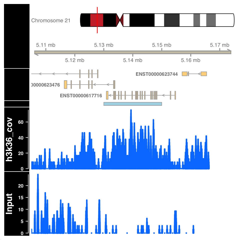
FIGURE 9.15: Visualization of H3K36me3 ChIP signal on a called broad peak.
Figure 9.15 shows a highly enriched H3K36me3 region covering the gene body, as expected.
9.6.4 Peak quality control
Peak calling is not a mathematically defined procedure; it is impossible to unambiguously define what a “peak” is. Therefore all of the peak calling procedures use heuristics, and statistical models which have been shown to work well in specific use cases. After peak calling, it is always necessary to check whether the defined peaks really are located in enriched regions, and in addition, use prior knowledge to ascertain whether the peaks correspond to known biology.
Peak calling can falsely identify enriched regions if the input sample is not sequenced to the proper depth. Because the input samples correspond to de facto whole genome sequencing, and the ChIP procedure enriches for a subset of the genome, it can often happen that many regions in the genome are not sufficiently covered by the Input sample. Such variability in the signal profile of Input samples can cause a region to be defined as a peak, enriched in the ChIP sample, while in reality it is depleted in the Input, due to under-sampling. For example, the figure in the previous chapter, showing an enriched region H3K36me3 over a gene body, shows a large depletion in the Input sample over the same region. Such depletion should be a concern and merit further investigation.
The quality of enrichment can be checked by calculating the percentage of reads within peaks for both ChIP and Input samples. ChIP samples should have a high percentage of reads in peaks, while for the input samples, the percentage of reads should correspond to the percentage of genome covered by peaks.
For transcription factor ChIP experiments, an important control is to determine whether the peak regions contain sequences which are known to be bound by the corresponding transcription factor - whether they contain known transcription factor binding motifs. Transcription factor binding motifs are sequence models which model the propensity of binding DNA sequences. Such sequence models can be downloaded from public databases and compared to see whether there is a positional enrichment around our peaks.
We will now calculate the percentage of reads within peaks for the H3K36me3 experiment. Subsequently, we will download the known CTCF sequence model, and compare it to our peak regions.
9.6.4.1 Percentage of reads in peaks
To calculate the reads in peaks, we will firstly extract the number of reads
in each tilling window from the normR produced fit object.
This is done using the getCounts() function.
We will then use the q-value to define which tilling windows correspond
to peaks, and count the number of reads within and outside peaks.
# extract, per tilling window, counts from the fit object
h3k36_counts = data.frame(getCounts(h3k36_fit))

# change the column names of the data.frame
colnames(h3k36_counts) = c('Input','H3K36me3')

# extract the q-value corresponding to each bin
h3k36_counts$qvalue = getQvalues(h3k36_fit)

# define which regions are peaks using a q value cutoff
h3k36_counts$enriched[is.na(h3k36_counts$qvalue)]  = 'Not Peak'
h3k36_counts$enriched[h3k36_counts$qvalue > 0.05]  = 'Not Peak'
h3k36_counts$enriched[h3k36_counts$qvalue <= 0.05] = 'Peak'

# remove the q value column
h3k36_counts$qvalue = NULL

# reshape the data.frame into a long format
h3k36_counts_df = tidyr::pivot_longer(
    data      = h3k36_counts,
    cols      = -enriched,
    names_to  = 'experiment',
    values_to = 'counts'
)

# sum the number of reads in the Peak and Not Peak regions
h3k36_counts_df = group_by(.data = h3k36_counts_df, experiment, enriched)
h3k36_counts_df = summarize(.data = h3k36_counts_df, num_of_reads = sum(counts))

# calculate the percentage of reads.
h3k36_counts_df       = group_by(.data = h3k36_counts_df, experiment)
h3k36_counts_df       = mutate(.data = h3k36_counts_df, total=sum(num_of_reads))
h3k36_counts_df$percentage = with(h3k36_counts_df, round(num_of_reads/total,2))
## # A tibble: 4 x 5
## # Groups: experiment [2]
## experiment enriched num_of_reads total percentage
## <chr> <chr> <int> <int> <dbl>
## 1 H3K36me3 Not Peak 67623 158616 0.43
## 2 H3K36me3 Peak 90993 158616 0.570
## 3 Input Not Peak 492369 648196 0.76
## 4 Input Peak 155827 648196 0.24We can now plot the percentage of reads in peaks:
ggplot(
    data = h3k36_counts_df,
    aes(
        x = experiment,
        y = percentage,
        fill = enriched
    )) +
    geom_bar(stat='identity', position='dodge') +
    theme_bw() +
    theme(
        axis.text = element_text(size=10, face='bold'),
        axis.title = element_text(size=12,face="bold"),
        plot.title = element_text(hjust = 0.5)) +
    xlab('Experiment') +
    ylab('Percetage of reads in region') +
    ggtitle('Percentage of reads in peaks for H3K36me3') +
    scale_fill_manual(values=c('gray','red'))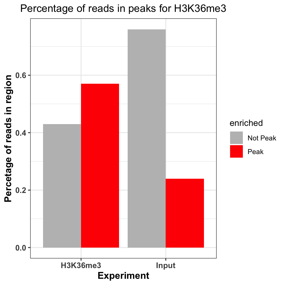
FIGURE 9.16: Percentage of ChIP reads in called peaks. Higher percentage indicates higher ChIP quality.
Figure 9.16 shows that the ChIP sample is clearly enriched in the peak regions. The percentage of reads in peaks will depend on the quality of the antibody (strength of enrichment), and the size of peaks which are bound by the protein of interest. If the total size of peaks is small, relative to the genome size, we can expect that the percentage of reads in peaks will be small.
9.6.4.2 DNA motifs on peaks
Well-studied transcription factors have publicly available transcription factor binding motifs. If such a model is available for our transcription factor of interest, we can use it to check the quality of our ChIP data. Two common measures are used for this purpose:
- Percentage of peaks containing the motif of interest.
- Positional distribution of the motif - the distribution of motif locations should be centered on the peak centers.
9.6.4.2.1 Representing motifs as matrices
In order to calculate the percentage of CTCF peaks which contain a known CTCF
motif. We need to find the CTCF motif and have the computational tools to search for that motif. The DNA binding motifs can be extracted from the MotifDB Bioconductor
database. The MotifDB is an agglomeration of multiple motif databases.
# load the MotifDB package
library(MotifDb)

# fetch the CTCF motif from the data base
motifs = query(query(MotifDb, 'Hsapiens'), 'CTCF')

# show all available ctcf motifs
motifs
## MotifDb object of length 12
## | Created from downloaded public sources: 2013-Aug-30
## | 12 position frequency matrices from 8 sources:
## | HOCOMOCOv10: 2
## | HOCOMOCOv11-core-A: 2
## | JASPAR_2014: 1
## | JASPAR_CORE: 1
## | SwissRegulon: 2
## | jaspar2016: 1
## | jaspar2018: 2
## | jolma2013: 1
## | 1 organism/s
## | Hsapiens: 12
## Hsapiens-SwissRegulon-CTCFL.SwissRegulon
## Hsapiens-SwissRegulon-CTCF.SwissRegulon
## Hsapiens-HOCOMOCOv10-CTCFL_HUMAN.H10MO.A
## Hsapiens-HOCOMOCOv10-CTCF_HUMAN.H10MO.A
## Hsapiens-HOCOMOCOv11-core-A-CTCFL_HUMAN.H11MO.0.A
## ...
## Hsapiens-JASPAR_2014-CTCF-MA0139.1
## Hsapiens-jaspar2016-CTCF-MA0139.1
## Hsapiens-jaspar2018-CTCF-MA0139.1
## Hsapiens-jaspar2018-CTCFL-MA1102.1
## Hsapiens-jolma2013-CTCFWe will extract the CTCF from the MotifDB (Khan, Fornes, Stigliani, et al. 2018) database.
# based on the MotifDB version, the location of the CTCF motif
# might change, if you do not get the expected results please try
# to subset with different indices
ctcf_motif  = motifs[[1]]
The motifs are usually represented as matrices of 4-by-N dimensions. In the matrix, each of 4 rows correspond to one nucleotide (A, C, G, T). The number of columns designates the width of the region bound by the transcription factor or the length of the motif that the protein recognizes. Each element of the matrix contains the probability of observing the corresponding nucleotide on this position. For example, for following the CTCF matrix in Table 9.1, the probability of observing a thymine at the first position of the motif,\(p_{i=1,k=4}\) , is 0.57 (1st column, 4th row). Such a matrix, where each column is a probability distribution over a sequence of nucleotides, is called a position frequency matrix (PFM). In some sources, this matrix is also called “position probability matrix (PPM)”. One way to construct such matrices is to get experimentally verified sequences that are bound by the protein of interest and then to use a motif-finding algorithm.
| 1 | 2 | 3 | 4 | 5 | 6 | 7 | 8 | 9 | 10 | 11 | 12 | 13 | 14 | 15 | 16 | 17 | 18 | 19 | 20 | |
|---|---|---|---|---|---|---|---|---|---|---|---|---|---|---|---|---|---|---|---|---|
| A | 0.17 | 0.23 | 0.29 | 0.10 | 0.33 | 0.06 | 0.05 | 0.04 | 0.02 | 0 | 0.25 | 0.00 | 0 | 0.05 | 0.25 | 0.00 | 0.17 | 0 | 0.02 | 0.19 |
| C | 0.42 | 0.28 | 0.30 | 0.32 | 0.11 | 0.33 | 0.56 | 0.00 | 0.96 | 1 | 0.67 | 0.69 | 1 | 0.04 | 0.07 | 0.42 | 0.15 | 0 | 0.06 | 0.43 |
| G | 0.25 | 0.23 | 0.26 | 0.27 | 0.42 | 0.55 | 0.05 | 0.83 | 0.01 | 0 | 0.03 | 0.00 | 0 | 0.02 | 0.53 | 0.55 | 0.05 | 1 | 0.87 | 0.15 |
| T | 0.16 | 0.27 | 0.15 | 0.31 | 0.14 | 0.06 | 0.33 | 0.13 | 0.00 | 0 | 0.06 | 0.31 | 0 | 0.89 | 0.15 | 0.03 | 0.62 | 0 | 0.05 | 0.23 |
Such a matrix can be used to calculate the probability that the transcription factor will bind to any given sequence. However, computationally, it is easier to work with summation rather than multiplication. In addition, the simple probabilistic model does not take the background probability of observing a certain base in a given position. We can correct for background base frequencies by dividing the individual probability, \(p_{i,k}\) in each cell of the matrix by the background base probability for a given base, \(B_k\). We can then take the logarithm of that quantity to calculate a log-likelihood and bring everything to log-scale as follows \(Score_{i,k}=log_2(p_{i,k}/B_k)\). We can now calculate a score for any given sequence by summing up the base-position-specific scores we obtain from the log-scaled matrix. This matrix is formally called position-specific scoring matrix (PSSM) or position-specific weight matrix (PWM). We can use this matrix to scan the genome in a sliding window manner and calculate a score for each window. Usually, a cutoff value is needed to call a motif hit. The higher the score you get from the PWM for a particular sequence, the better it is. The traditional algorithms we will use in the following sections use 80% of the maximum rescaled score you can obtain from a PWM as the default cutoff for a hit. The rescaling is simple min-max rescaling where you rescale the score by subtracting the minimum score and dividing that by \(max(PWMscore)-min(PWMscore)\). The motif scanning approach is illustrated in Figure 9.17. In this example, ACACT is not considered a hit because its score only corresponds to only \(15.6\) % of the rescaled maximum score.
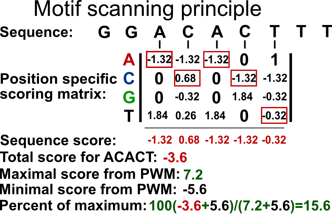
FIGURE 9.17: PWM scanning principle. A genomic sequence is scanned by a PWM matrix. This matrix is used to measure how likely it is that the transcription factor will bind each nucleotide in each position. Here we are looking at how likely it is that our TF will bind to the sequence ACACT. The score for this sequence is -3.6. The maximal score obtainable by the PWM is 7.2 and minimum is -5.6. After min-max rescaling, -3.6 corresponds to a 15% score and ACACT is not considered a hit.
9.6.4.2.2 Representing motifs as sequence logos
Using the PFM, we can calculate the information content of each position in the matrix. The information content quantifies the contribution of each nucleotide to the cumulative binding preference. This tells us how important each nucleotide is for the binding. It additionally allows us to visually represent the probability matrices as sequence logos. The information content is quantified as relative entropy. It ranges from \(0\), no information, to \(2\), maximal information. For a column in the PFM, the entropy is calculated as follows:
\[ entropy = -\sum\limits_{k=1}^n p_{i,k}\log_2(p_{i,k}) \] \(p_{i,k}\) is the probability of observing base \(k\) in the column \(i\) of the PFM. In other words, \(p_{i,k}\) is simply the value of the cell in the PFM. The entropy value is high when the probabilities of each base are similar and low when it is much more probable that only one base occur in a given column. The relative portion comes from the fact that we compare the entropy we calculated for a column to the maximum entropy we can obtain. If the all bases are equally likely for a position in the PFM, then we will have the maximum entropy and we compare our original entropy to that maximum entropy. The maximum entropy is simply \(log_2{n}\) where \(n\) is number of letters in the alphabet. In our case we have 4 letters A,C,G and T. The information content is then simply subtracting the observed entropy for a column from the maximum entropy, which translates to the following equation:
\[ IC=log_2(n)+\sum\limits_{k=1}^n p_{i,k}\log_2(p_{i,k}) \] The information content, \(IC\), in the preceding equation, will be high if a base has a high probability of occurrence and low if all bases are more or less equally likely to occur.
We can visualize the matrix by visualizing the letters weighted by their probabilities in the PFM. This approach is shown on the left-hand side of Figure 9.18. In addition, we can also calculate the information content per column to weight the probabilities. This means that the columns that have very frequent letters will be higher. This approach is shown on the right-hand side of Figure 9.18. We will use below the seqLogo package to visualize the CTCF motif in the two different ways we described above.
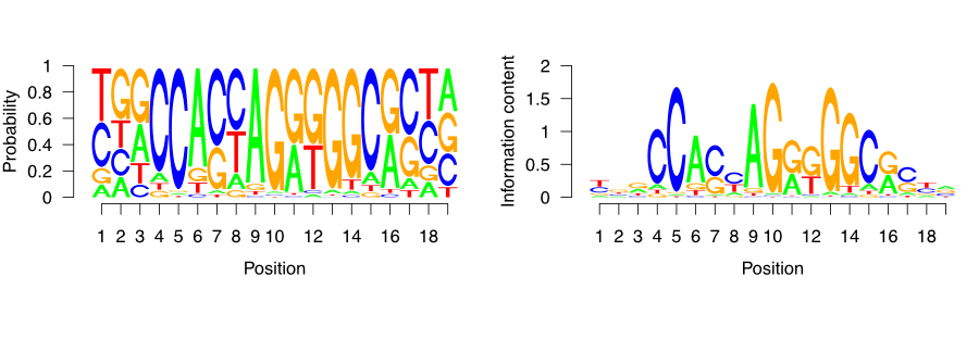
FIGURE 9.18: CTCF sequence motif visualized as a sequence logo. Y-axis ranges from zero to two, and corresponds to the amount of information each base in the motif contributes to the overall motif. The larger the letter, the greater the probability of observing just one defined base on the designated position.
9.6.4.2.3 Percentage of peaks with the motif
Since we now understand how DNA motifs are used we can start annotating the CTCF peaks with the motif. First, we will extend the peak regions to +/- 200 bp around the peak center. Because the average fragment size is 200 bp, 400 nucleotides is the expected variation in the position of the true binding location.
Now we use the BSgenome package to
extract the sequences corresponding to the peak regions.
# load the human genome sequence
library(BSgenome.Hsapiens.UCSC.hg38)

# extract the sequences around the peaks
seq = getSeq(BSgenome.Hsapiens.UCSC.hg38, ctcf_peaks_resized)
Once we have extracted the sequences, we can use the CTCF motif to
scan each sequence and determine the probability of CTCF binding.
For this we use the TFBSTools (Tan and Lenhard 2016) package.
We first convert the raw probability matrix into a PWMMatrix object,
which can then be used for efficient scanning.
# load the TFBS tools package
library(TFBSTools)

# convert the matrix into a PWM object
ctcf_pwm = PWMatrix(
    ID = 'CTCF',
    profileMatrix = ctcf_motif
)
We can now use the searchSeq() function to scan each sequence for the motif occurrence.
Because the motif matrices are given a continuous binding score, we need to set a cutoff to
determine when a sequence contains the motif, and when it doesn’t.
The cutoff is set by determining the maximal possible score produced by the motif matrix;
a percentage of that score is then taken as the threshold value.
For example, if the best sequence would have a score of 1.4 of being bound,
then we define a threshold of 80% of 1.4, which is 1.12; and any sequence which
scores less than 1.12 would not be marked as being bound by the protein.
For the CTCF, we mark any peak containing a sequence with > 80% of the maximal rescaled score or “relative score” as a positive hit.
##   seqnames source feature start end absScore relScore strand   ID
## 1        1   TFBS    TFBS    44  63     11.9    0.921      - CTCF
## 2        1   TFBS    TFBS   102 121     11.0    0.839      - CTCF
## 3        2   TFBS    TFBS   151 170     11.5    0.881      + CTCF
## 4        4   TFBS    TFBS   294 313     11.9    0.921      - CTCF
## 5        4   TFBS    TFBS   352 371     11.0    0.839      - CTCF
## 6        5   TFBS    TFBS   164 183     10.9    0.831      - CTCF
A common diagnostic plot is to graph a reverse cumulative distribution of peak occurrences. On the x-axis we rank the peaks, with the most highly enriched peak in the first position, and the least enriched peak in the last position. We then walk from the lowest to the highest ranking and measure the percentage of peaks containing the motif.
# label which peaks contain CTCF motifs
motif_hits_df = data.frame(
  peak_order     = 1:length(ctcf_peaks)
)
motif_hits_df$contains_motif = motif_hits_df$peak_order %in% hits$seqnames
motif_hits_df = motif_hits_df[order(-motif_hits_df$peak_order),]

# calculate the percentage of peaks with motif for peaks of descending strength
motif_hits_df$perc_peaks = with(motif_hits_df,
                                cumsum(contains_motif) / max(peak_order))
motif_hits_df$perc_peaks = round(motif_hits_df$perc_peaks, 2)
We can now visualize the percentage of peaks with matching CTCF motif.
# plot the cumulative distribution of motif hit percentages
ggplot(
    motif_hits_df,
    aes(
        x = peak_order,
        y = perc_peaks
    )) +
  geom_line(size=2) +
  theme_bw() +
  theme(
    axis.text = element_text(size=10, face='bold'),
    axis.title = element_text(size=14,face="bold"),
    plot.title = element_text(hjust = 0.5)) +
  xlab('Peak rank') +
  ylab('Percetage of peaks with motif') +
  ggtitle('Percentage of CTCF peaks with the CTCF motif')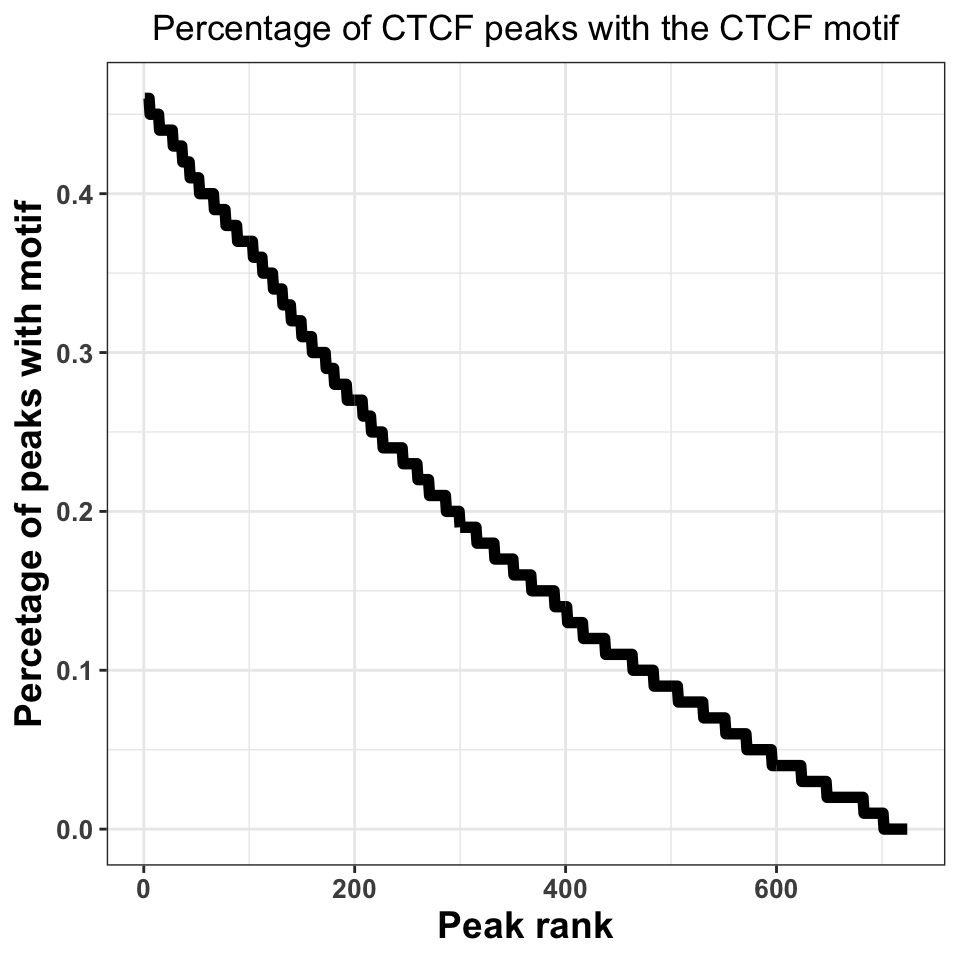
FIGURE 9.19: Percentage of peaks containing the motif. Higher percentage indicates a better ChIP-experiment, and a better peak calling procedure.
Figure 9.19 shows that, when we take all peaks into account, ~45% of the peaks contain a CTCF motif. This is an excellent percentage and indicates a high-quality ChIP experiment. Our inability to locate the motif in ~50% of the sequences does not necessarily need to be a consequence of a poor experiment; sometimes it is a result of the molecular mechanism by which the transcription factor binds. If a transcription factor has multiple binding modes, which are context dependent, for example, if the transcription factor binds indirectly to a subset of regions, through an interacting partner, we do not have to observe a motif.
9.6.4.3 Motif localization
If the ChIP experiment was performed properly, we would expect the motif to be localized just below the summit of each peak. By plotting the motif localization around ChIP peaks, we are quantifying the uncertainty in the peak location.
We will firstly resize our peaks into regions around +/−1-kb around the peak center.
# resize the region around peaks to +/- 1kb
ctcf_peaks_resized = resize(ctcf_peaks, width = 2000, fix='center')
Now we perform the motif localization, as before.
# fetch the sequence
seq = getSeq(BSgenome.Hsapiens.UCSC.hg38,ctcf_peaks_resized)

# convert the motif matrix to PWM, and scan the peaks
ctcf_pwm    = PWMatrix(ID = 'CTCF', profileMatrix = ctcf_motif)
hits = searchSeq(ctcf_pwm, seq, min.score="80%", strand="*")
hits = as.data.frame(hits)
We now construct a plot, where the X-axis represents the +/- 1000 nucleotides around the peak, while the Y-axis shows the motif enrichment at each position.
# set the position relative to the start
hits$position = hits$start - 1000

# plot the motif hits around peaks
ggplot(data=hits, aes(position)) +
  geom_density(size=2) +
  theme_bw() +
  geom_vline(xintercept = 0, linetype=2, color='red', size=2) +
  xlab('Position around the CTCF peaks') +
  ylab('Per position percentage\nof motif occurence') +
  theme(
    axis.text = element_text(size=10, face='bold'),
    axis.title = element_text(size=14,face="bold"),
    plot.title = element_text(hjust = 0.5))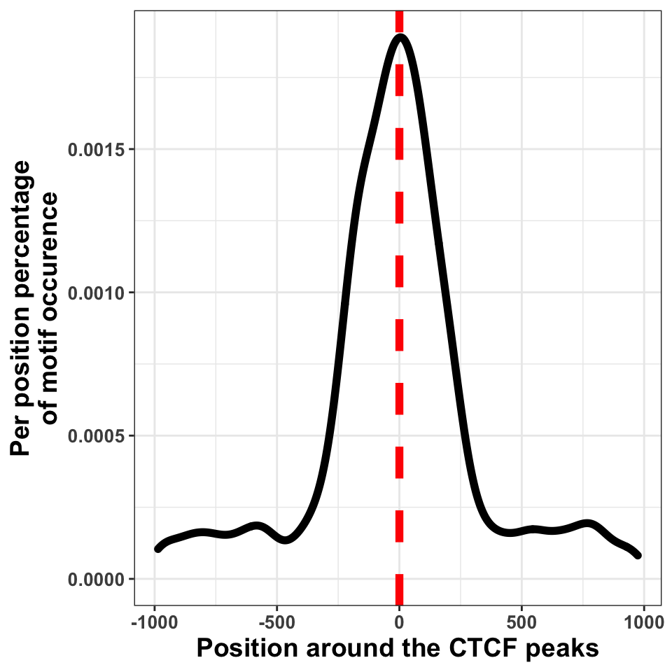
FIGURE 9.20: Transcription factor sequence motif localization with respect to the defined binding sites.
We can in Figure 9.20, see that the bulk of motif hits are found in a region of \(+/-\) 250 bp around the peak centers. This means that the peak calling procedure was quite precise.
9.6.5 Peak annotation
As the final step of quality control we will visualize the distribution of peaks in different functional genomic regions. The purpose of the analysis is to check whether the location of the peaks conforms our prior knowledge. This analysis is equivalent to constructing distributions for reads.
Firstly we download the human gene models and construct the annotation hierarchy.
# download the annotation
hub = AnnotationHub()
gtf = hub[['AH61126']]
seqlevels(gtf, pruning.mode='coarse') = '21'
seqlevels(gtf, pruning.mode='coarse') = paste0('chr', seqlevels(gtf))

# create the annotation hierarchy
annotation_list = GRangesList(
  tss    = promoters(subset(gtf, type=='gene'), 1000, 1000),
  exon   = subset(gtf, type=='exon'),
  intron = subset(gtf, type=='gene')
)
The following function finds the genomic location of each peak, annotates the peaks using the hierarchical prioritization, and calculates the summary statistics.
The function contains four major parts:
- Creating a disjoint set of peak regions.
- Finding the overlapping annotation for each peak.
- Annotating each peak with the corresponding annotation class.
- Calculating summary statistics
# function which annotates the location of each peak
annotatePeaks = function(peaks, annotation_list, name){

  # ------------------------------------------------ #
  # 1. getting disjoint regions
  # collapse touching enriched regions
  peaks = reduce(peaks)

  # ------------------------------------------------ #
  # 2. overlapping peaks and annotation
  # find overlaps between the peaks and annotation_list
  result = as.data.frame(findOverlaps(peaks, annotation_list))

  # ------------------------------------------------ #
  # 3. annotating peaks
  # fetch annotation names
  result$annotation = names(annotation_list)[result$subjectHits]

  # rank by annotation precedence
  result = result[order(result$subjectHits),]

  # remove overlapping annotations
  result = subset(result, !duplicated(queryHits))

  # ------------------------------------------------ #
  # 4. calculating statistics
  # count the number of peaks in each annotation category
  result = group_by(.data = result, annotation)
  result = summarise(.data = result, counts = length(annotation))

  # fetch the number of intergenic peaks
  result = rbind(result,
                 data.frame(annotation = 'intergenic',
                            counts     = length(peaks) - sum(result$counts)))

  result$frequency  = with(result, round(counts/sum(counts),2))
  result$experiment = name

  return(result)
}
Using the above defined annotatePeaks() function we will now annotate CTCF
and H3K36me3 peaks. Firstly we create a list which contains both CTCF and H3K36me3 peaks.
Using the lapply() function we apply the annotatePeaks() function
on each element of the list.
# calculate the distribution of peaks in annotation for each experiment
annot_peaks_list = lapply(names(peak_list), function(peak_name){
  annotatePeaks(peak_list[[peak_name]], annotation_list, peak_name)
})
We use the dplyr::bind_rows() function to combine the CTCF and H3K36me3 annotation
statistics into one data frame.
# combine a list of data.frames into one data.frame
annot_peaks_df = dplyr::bind_rows(annot_peaks_list)
And visualize the results as bar plots. Resulting plot is in Figure 9.21, which shows that the H3K36me3 peaks are located preferentially in gene bodies, as expected, while the CTCF peaks are found preferentially in introns.
# plot the distribution of peaks in genomic features
ggplot(data = annot_peaks_df,
       aes(
           x    = experiment,
           y    = frequency,
           fill = annotation
        )) +
  geom_bar(stat='identity') +
  scale_fill_brewer(palette='Set2') +
  theme_bw()+
  theme(
    axis.text = element_text(size=18, face='bold'),
    axis.title = element_text(size=14,face="bold"),
    plot.title = element_text(hjust = 0.5))  +
  ggtitle('Peak distribution in\ngenomic regions') +
  xlab('Experiment') +
  ylab('Frequency')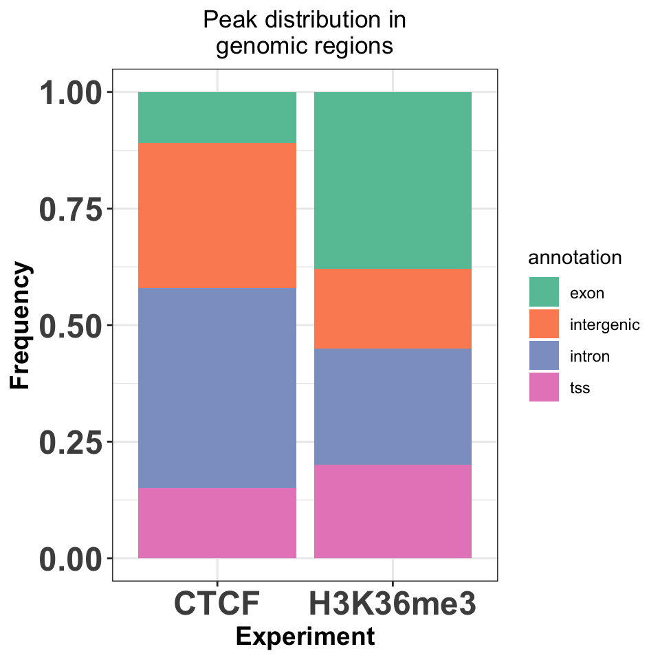
FIGURE 9.21: Enrichment of transcription factor or histone modifications in functional genomic features.
References
Beck, Brandl, Boelen, Unnikrishnan, Pimanda, and Wong. 2012. “Signal Analysis for Genome-Wide Maps of Histone Modifications Measured by ChIP-Seq.” Bioinformatics 28 (8): 1062–9. https://doi.org/10.1093/bioinformatics/bts085.
Han, Tian, Pécot, Huang, Machiraju, and Huang. 2012. “A Signal Processing Approach for Enriched Region Detection in RNA Polymerase II ChIP-Seq Data.” BMC Bioinformatics 13 Suppl 2 (March): S2. https://doi.org/10.1186/1471-2105-13-S2-S2.
Helmuth, Li, Arrigoni, et al. 2016. “normR: Regime Enrichment Calling for ChIP-Seq Data.” bioRxiv.
Khan, Fornes, Stigliani, et al. 2018. “JASPAR 2018: Update of the Open-Access Database of Transcription Factor Binding Profiles and Its Web Framework.” Nucleic Acids Res 46 (D1): D260–D266. https://doi.org/10.1093/nar/gkx1126.
Laajala, Raghav, Tuomela, Lahesmaa, Aittokallio, and Elo. 2009. “A Practical Comparison of Methods for Detecting Transcription Factor Binding Sites in ChIP-Seq Experiments.” BMC Genomics 10 (December): 618. https://doi.org/10.1186/1471-2164-10-618.
Micsinai, Parisi, Strino, Asp, Dynlacht, and Kluger. 2012. “Picking ChIP-Seq Peak Detectors for Analyzing Chromatin Modification Experiments.” Nucleic Acids Res 40 (9): e70. https://doi.org/10.1093/nar/gks048.
Rashid, Giresi, Ibrahim, Sun, and Lieb. 2011. “ZINBA Integrates Local Covariates with DNA-Seq Data to Identify Broad and Narrow Regions of Enrichment, Even Within Amplified Genomic Regions.” Genome Biol 12 (7): R67. https://doi.org/10.1186/gb-2011-12-7-r67.
Shao, Zhang, Yuan, Orkin, and Waxman. 2012. “MAnorm: A Robust Model for Quantitative Comparison of ChIP-Seq Data Sets.” Genome Biol 13 (3): R16. https://doi.org/10.1186/gb-2012-13-3-r16.
Song, and Smith. 2011. “Identifying Dispersed Epigenomic Domains from ChIP-Seq Data.” Bioinformatics 27 (6): 870–71. https://doi.org/10.1093/bioinformatics/btr030.
Tan, and Lenhard. 2016. “TFBSTools: An R/Bioconductor Package for Transcription Factor Binding Site Analysis.” Bioinformatics 32 (10): 1555–6. https://doi.org/10.1093/bioinformatics/btw024.
Wilbanks, and Facciotti. 2010. “Evaluation of Algorithm Performance in ChIP-Seq Peak Detection.” PLoS ONE 5 (7): e11471. https://doi.org/10.1371/journal.pone.0011471.
Xing, Mo, Liao, and Zhang. 2012. “Genome-Wide Localization of Protein-DNA Binding and Histone Modification by a Bayesian Change-Point Method with ChIP-Seq Data.” PLoS Comput Biol 8 (7): e1002613. https://doi.org/10.1371/journal.pcbi.1002613.
Xu, Handoko, Wei, Ye, Sheng, Wei, Lin, and Sung. 2010. “A Signal-Noise Model for Significance Analysis of ChIP-Seq with Negative Control.” Bioinformatics 26 (9): 1199–1204. https://doi.org/10.1093/bioinformatics/btq128.
Zang, Schones, Zeng, Cui, Zhao, and Peng. 2009. “A Clustering Approach for Identification of Enriched Domains from Histone Modification ChIP-Seq Data.” Bioinformatics 25 (15): 1952–8. https://doi.org/10.1093/bioinformatics/btp340.
Zhang, Liu, Meyer, et al. 2008. “Model-Based Analysis of ChIP-Seq (MACS).” Genome Biol 9 (9): R137. https://doi.org/10.1186/gb-2008-9-9-r137.