5.12 Trees and forests: Random forests in action
5.12.1 Decision trees
Decision trees are a popular method for various machine learning tasks mostly because their interpretability is very high. A decision tree is a series of filters on the predictor variables. The series of filters end up in a class prediction. Each filter is a binary yes/no question, which creates bifurcations in the series of filters thus leading to a treelike structure. The filters are dependent on the type of predictor variables. If the variables are categorical, such as gender, then the filters could be “is gender female” type of questions. If the variables are continuous, such as gene expression, the filter could be “is PIGX expression larger than 210?”. Every point where we filter samples based on these questions are called “decision nodes”. The tree-fitting algorithm finds the best variables at decision nodes depending on how well they split the samples into classes after the application of the decision node. Decision trees handle both categorical and numeric predictor variables, they are easy to interpret, and they can deal with missing variables. Despite their advantages, decision trees tend to overfit if they are grown very deep and can learn irregular patterns. There are many variants of tree-based machine learning algorithms. However, most algorithms construct decision nodes in a top down manner. They select the best variables to use in decision nodes based on how homogeneous the sample sets are after the split. One measure of homogeneity is “Gini impurity”. This measure is calculated for each subset after the split and later summed up as a weighted average. For a decision node that splits the data perfectly in a two-class problem, the gini impurity will be \(0\), and for a node that splits the data into a subset that has 50% class A and 50% class B the impurity will be \(0.5\). Formally, the gini impurity, \({I}_{G}(p)\), of a set of samples with known class labels for \(K\) classes is the following, where \(p_{i}\) is the probability of observing class \(i\) in the subset:
\[ {\displaystyle {I}_{G}(p)=\sum _{i=1}^{K}p_{i}(1-p_{i})=\sum _{i=1}^{K}p_{i}-\sum _{i=1}^{K}{p_{i}}^{2}=1-\sum _{i=1}^{K}{p_{i}}^{2}} \]
For example, if a subset of data after split has 75% class A and 25% class B for that subset, the impurity would be \(1-(0.75^2+0.25^2)=0.375\). If the other subset had 5% class A and 95% class B, its impurity would be \(1-(0.95^2+0.05^2)=0.095\). If the subset sizes after the split were equal, total weighted impurity would be \(0.5*0.375+0.5*0.095= 0.235\). These calculations will be done for each potential variable and the split, and every node will be constructed based on gini impurity decrease. If the variable is continuous, the cutoff value will be decided based on the best impurity. For example, gene expression values will have splits such as “PIGX expression < 2.1”. Here \(2.1\) is the cutoff value that produces the best impurity. There are other homogeneity measures, however gini impurity is the one that is used for random forests, which we will introduce next.
5.12.2 Trees to forests
Random forests are devised to counter the shortcomings of decision trees. They are simply ensembles of decision trees. Each tree is trained with a different randomly selected part of the data with randomly selected predictor variables. The goal of introducing randomness is to reduce the variance of the model so it does not overfit, at the expense of a small increase in the bias and some loss of interpretability. This strategy generally boosts the performance of the final model.
The random forests algorithm tries to decorrelate the trees so that they learn different things about the data. It does this by selecting a random subset of variables. If one or a few predictor variables are very strong predictors for the response variable, these features will be selected in many of the trees, causing them to become correlated. Random subsampling of predictor variables ensures that not always the best predictors overall are selected for every tree and, the model does have a chance to learn other features of the data.
Another sampling method introduced when building random forest models is bootstrap resampling before constructing each tree. This brings the advantage of out-of-the-bag (OOB) error prediction. In this case, the prediction error can be estimated for training samples that were OOB, meaning they were not used in the training, for some percentage of the trees. The prediction error for each sample can be estimated from the trees where that sample was OOB. OOB estimates claimed to be a good alternative to cross-validation estimated errors (Breiman 2001).
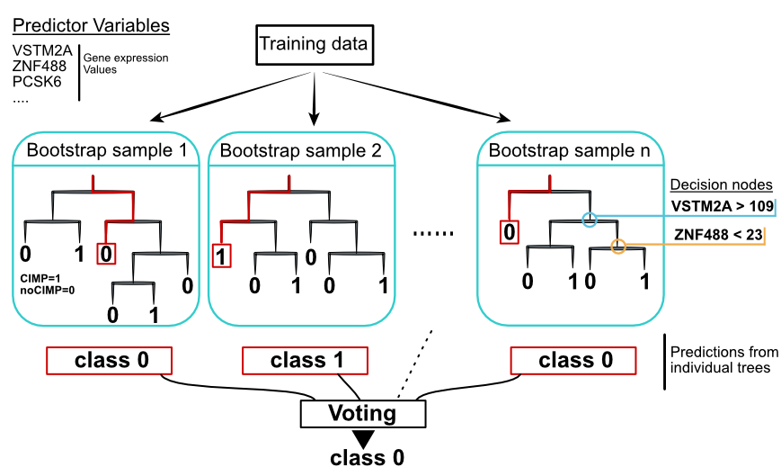
FIGURE 5.9: Random forest concept. Individual decision trees are built with sampling strategies. Votes from each tree define the final class.
For demonstration purposes, we will use the caret package interface to the ranger random forest package. This is a fast implementation of the original random forest algorithm. For random forests, we have two critical arguments. One of the most critical arguments for random forest is the number of predictor variables to sample in each split of the tree. This parameter controls the independence between the trees, and as explained before, this limits overfitting. Below, we are going to fit a random forest model to our tumor subtype problem. We will set mtry=100 and not perform the training procedure to find the best mtry value for simplicity. However, it is good practice
to run the model with cross-validation and let it pick the best parameters based on the cross-validation performance. It defaults to the square root of number of predictor variables. Another variable we can tune is the minimum node size of terminal nodes in the trees (min.node.size). This controls the depth of the trees grown. Setting this to larger numbers might cost a small loss in accuracy but the algorithm will run faster.
set.seed(17)

# we will do no resampling based prediction error
# although it is advised to do so even for random forests
trctrl <- trainControl(method = "none")

# we will now train random forest model
rfFit <- train(subtype~.,
               data = training,
               method = "ranger",
               trControl=trctrl,
               importance="permutation", # calculate importance
               tuneGrid = data.frame(mtry=100,
                                     min.node.size = 1,
                                     splitrule="gini")
               )
# print OOB error
rfFit$finalModel$prediction.error
## [1] 0.015384625.12.3 Variable importance
Random forests come with built-in variable importance metrics. One of the metrics is similar to the “variable dropout metric” where the predictor variables are permuted. In this case, OOB samples are used and the variables are permuted one at a time. Every time, the samples with the permuted variables are fed to the network and the decrease in accuracy is measured. Using this quantity, the variables can be ranked.
A less costly method with similar performance is to use gini impurity. Every time a variable is used in a tree to make a split, the gini impurity is less than the parent node. This method adds up these gini impurity decreases for each individual variable across the trees and divides it by the number of the trees in the forest. This metric is often consistent with the permutation importance measure (Breiman 2001). Below, we are going to plot the permutation-based importance metric. This metric has been calculated during the run of the model above. We will use the caret::varImp() function to access the importance values and plot them using the plot() function; the result is shown in Figure 5.10.
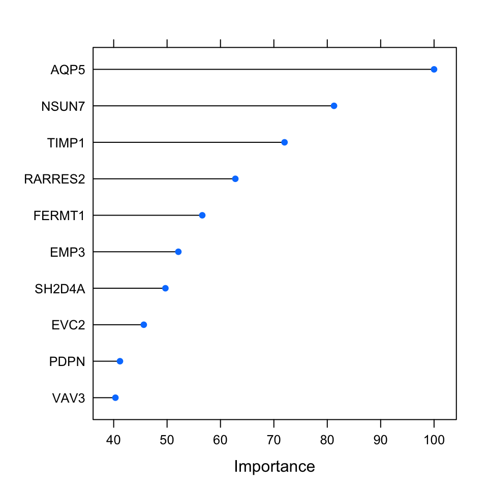
FIGURE 5.10: Top 10 important variables based on permutation-based method for the random forest classification.
References
Breiman. 2001. “Random Forests.” Machine Learning 45 (1): 5–32.